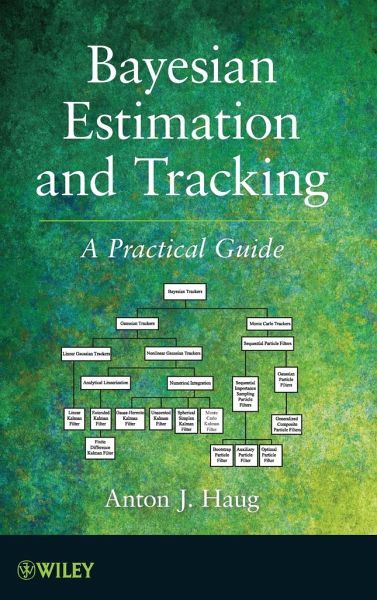
Anton J. Haug

Bayesian Estimation

• Gebundenes Buch

Produktbeschreibung

This book presents a practical approach to estimation methods that are designed to provide a clear path to programming all algorithms. Readers are provided with a firm understanding of Bayesian estimation methods and their interrelatedness. Starting with fundamental principles of Bayesian theory, the book shows how each tracking filter is derived from a slight modification to a previous filter. Such a development gives readers a broader understanding of the hierarchy of Bayesian estimation and tracking. Following the discussions about each tracking filter, the filter is put into block diagram form for ease in future recall and reference. The book presents a completely unified approach to Bayesian estimation and tracking, and this is accomplished by showing that the current posterior density for a state vector can be linked to its previous posterior density through the use of Bayes' Law and the Chapman-Kolmogorov integral. Predictive point estimates are then shown to be density-weighted integrals of nonlinear functions. The book also presents a methodology that makes implementation of the estimation methods simple (or, rather, simpler than they have been in the past). Each algorithm is accompanied by a block diagram that illustrates how all parts of the tracking filter are linked in a never-ending chain, from initialization to the loss of track. These filter block diagrams provide a ready picture for implementing the algorithms into programmable code. In addition, four completely worked out case studies give readers examples of implementation, from simulation models that generate noisy observations to worked-out applications for all tracking algorithms. This book also presents the development and application of track performance metrics, including how to generate error ellipses when implementing in real-world applications, how to calculate RMS errors in simulation environments, and how to calculate Cramer-Rao lower bounds for the RMS errors. These are also illustrated in the case study presentations.

---

A practical approach to estimating and tracking dynamic systems in real-worl applications

Much of the literature on performing estimation for non-Gaussian systems is short on practical methodology, while Gaussian methods often lack a cohesive derivation. Bayesian Estimation and Tracking addresses the gap in the field on both accounts, providing readers with a comprehensive overview of methods for estimating both linear and nonlinear dynamic systems driven by Gaussian and non-Gaussian noices.

Featuring a unified approach to Bayesian estimation and tracking, the book emphasizes the derivation of all tracking algorithms within a Bayesian framework and describes effective numerical methods for evaluating density-weighted integrals, including linear and nonlinear Kalman filters for Gaussian-weighted integrals and particle filters for non-Gaussian cases. The author first emphasizes detailed derivations from first principles of eeach estimation method and goes on to use illustrative and detailed step-by-step instructions for each method that makes coding of the tracking filter simple and easy to understand.

Case studies are employed to showcase applications of the discussed topics. In addition, the book supplies block diagrams for each algorithm, allowing readers to develop their own MATLAB(r) toolbox of estimation methods.

Bayesian Estimation and Tracking is an excellent book for courses on estimation and tracking methods at the graduate level. The book also serves as a valuable reference for research scientists, mathematicians, and engineers seeking a deeper understanding of the topics.

Produktdetails

• Verlag: Wiley & Sons
• Artikelnr. des Verlages: 14562170000
• 1. Auflage
• Seitenzahl: 400
• Erscheinungstermin: 4. Juni 2012
• Englisch
• Abmessung: 240mm x 161mm x 26mm
• Gewicht: 690g
• ISBN-13: 9780470621707
• ISBN-10: 0470621702
• Artikelnr.: 35046491

Autorenporträt

ANTON J. HAUG, PhD, is member of the technical staff at the Applied Physics Laboratory at The Johns Hopkins University, where he develops advanced target tracking methods in support of the Air and Missile Defense Department. Throughout his career, Dr. Haug has worked across diverse areas such as target tracking; signal and array processing and processor design; active and passive radar and sonar design; digital communications and coding theory; and time- frequency analysis.

Inhaltsangabe

Preface Acknowledgments List of Figures xi List of Tables xxi Part I.
Prelininaries 1. Introduction 3 1.1 Bayesian Inference 5 1.2 Bayesian
Hierarchy of Estimation Methods 7 1.3 Scope of this Text 8 1.4 Modeling and
Simulation with Matlab(r) 13 2. Preliminary Mathematical Concepts 19 2.1 A
Very Brief Overview of Matrix Linear Algebra 20 2.2 Vector Point Generators
27 2.3 Approximating Nonlinear Multidimensional Functions with
Multidimensional Arguments 32 2.4 Overview of Multivariate Statistics 47 3.
General Concepts of Bayesian Estimation 69 3.1 Bayesian Estimation 70 3.2
Point Estimators 72 3.3 Introduction to Recursive Bayesian Filtering of
Probability Density Functions 76 3.4 Introduction to Recursive Bayesian
Estimation of the State Mean and Covariance 81 3.5 Discussion of General
Estimation Methods 88 4. Case Studies: Preliminary Discussions 93 4.1 The
Overall Simulation/Estimation/Evaluation Process 94 4.2 A Scenario
Simulator for Tracking a Constant-Velocity Target Through a DIFAR Buoy
Field 97 4.3 DIFAR Buoy Signal Processing 102 4.4 The DIFAR Likelihood
Function 111 Part II. The Gaussian Assumption: A Family of Kalman Filter
Estimators 5. The Gaussian Noise Case: Multidimensional Integration of
Gaussian-Weighted Distributions 119 5.1 Summary of Important Results From
Chapter 3 122 5.2 Derivation of the Kalman Filter Correction (Update)
Equations Revisted 124 5.3 The General Bayesian Point Prediction Integrals
for Gaussian Densities 128 6. The Linear Class of Kalman Filters 141 6.1
Linear Dynamic Models 142 6.2 Linear Observation Models 143 6.3 The Linear
Kalman Filter 144 6.4 Application of the LKF to DIFAR Buoy Bearing
Estimation 146 7. The Analytical Linearization Class of Kalman Filters: The
Extended Kalman Filter 153 7.1 One-Dimensional Consideration 154 7.2
Multidimensional Consideration 159 7.3 An Alternate Derivation of the
Multidimensional Covariance Prediction Equations 172 7.4 Application of the
EKF to the DIFAR Ship Tracking Case Study 174 8. The Sigma Point Class: The
Finite Difference Kalman Filter 187 8.1 One-Dimensional Finite Difference
Kalman Filter 189 8.2 Multidimensional Finite Difference Kalman Filters 195
8.3 An Alternate Derivation of the Multidimensional Finite Difference
Covariance Prediction Equations 201 9. The Sigma Point Class: The Unscented
Kalman Filter 207 9.1 Introduction to Monomial Cubature Integration Rules
207 9.2 The Unscented Kalman Filter 211 9.3 Applications of the UKF to the
DIFAR Ship Tracking Case Study 221 10. The Sigma Point Class: The Spherical
Simplex Kalman Filter 227 10.1 One-Dimensional Spherical Simplex Sigma
Points 228 10.2 Two-Dimensional Spherical Simplex Sigma Points 229 10.3
Higher-Dimensional Spherical Simplex Sigma Points 233 10.4 The Spherical
Simplex Kalman Filter 233 10.5 The Spherical Simplex Kalman Filter Process
236 10.6 Application of the SSKF to the DIFAR Ship Tracking Case Study 236
11. The Sigma Point Class: The Gauss-Hermite Kalman Filter 241 11.1
One-Dimensional Gauss-Hermite Quadrature 242 11.2 One-Dimensional
Gauss-Hermite Kalman Filter 248 11.3 Multidimensional Gauss-Hermite Kalman
Filter 251 11.4 Sparse Grid Approximation for High Dimension/High
Polynomial Order 257 11.5 Application of the GHKF to the DIFAR Ship
Tracking Case Study 261 12. The Monte Carlo Kalman Filter 265 12.1 The
Monte Carlo Kalman Filter 268 13. Summary of Gaussian Kalman Filters 273
13.1 Analytical Kalman Filters 274 13.2 Sigma-Point Kalman Filters 276 13.3
A More Practical Approach to Utilizing the Family of Kalman Filters 284 14.
Performance Measures for the Family of Kalman Filters 289 14.1 Error
Ellipses 290 14.2 Root Mean Squared Errors 299 14.3 Divergent Tracks 301
14.4 Cramer-Rao Lower Bound 302 14.5 Performance of Kalman Class DIFAR
Track Estimators 315 Part III. Monte Carlo Methods 15. Introduction to
Monte Carlo Methods 323 15.1 Approximating a Density From a Set of Monte
Carlo Samples 325 15.2 General Concepts Importance Sampling 340 15.3
Summary 347 16. Sequential Importance Sampling Particle Filters 351 16.1
General Concept of Sequential Importance Sampling 351 16.2 Resampling and
Regularization (Move) for SIS Particle Filters 357 16.3 The Bootstrap
Particle Filter 372 16.4 The Optimal SIS Particle Filter 378 16.5 The SIS
Auxiliary Particle Filter 385 16.6 Approximations to the SIS Auxiliary
Particle Filter 393 16.7 Reducing the Computational Load Through
Rao-Blackwellization 396 17. The Generalized Sequential Monte Carlo
Particle Filter 403 17.1 The Gaussian Particle Filter 404 17.2 The
Combination Particle Filter 406 17.3 Performance Comparison of all DIFAR
Tracking Filters 411 Part IV Additional Case Studies 18. A Spherical
Constant Velocity Model for Target Tracking in Three Dimensions 421 18.1
Tracking a Target in Cartesian Coordinates 426 18.2 Tracking a Target in
Spherical Coordinates 433 18.3 Implementation of Cartesian and Spherical
Tracking Filters 443 18.4 Performance Comparison for Various Estimation
Methods 453 18.5 Some Observations and Future Considerations 469 19.
Tracking a Falling Rigid Body Using Photogrammetry 497 19.1 Introduction
497 19.2 The Process (Dynamic) Model for Rigid Body Motion 502 19.3
Components of the Observation Model 513 19.4 Estimation Methods 517 19.5
The Generation of Synthetic Data 529 19.6 Performance Comparison Analysis
538 20. Sensor Fusion using Photogrammetric and Inertial Measurements 559
20.1 Introduction 559 20.2 The Process (Dynamic) Model for Rigid Body
Motion 562 20.3 The Sensor Fusion Observational Model563 20.4 The
Generation of Synthetic Data 569 20.5 Estimation Methods 572 20.6
Performance Comparison Analysis 577 20.7 Conclusions 585 20.8 Future Work
586 References 589