Mark W.J. Blok, A.T. Kearney

Dynamic Models of the Firm

Determining Optimal Investment, Financing and Production Policies by Computer

• Broschiertes Buch

Produktbeschreibung

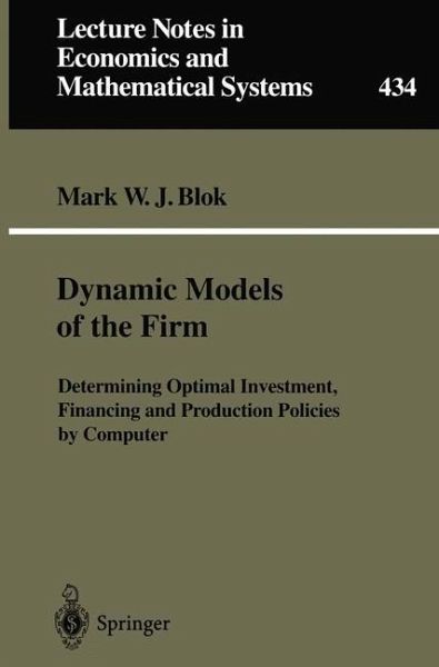
The research described in this book contributes to the scientific field of optimal control theory applied to dynamic models of the firm. In 1963, Jorgenson first wrote about the use of optimal control theory in order to analyze the dynamic investment behaviour of a hypothetical firm. A decade later, reports appeared of work on more realistic models of the firm carried out by, amongst others, Lesourne [1973) and Bensoussan et al. [1974). In The Netherlands, P. A. Verheyen, Professor of Management Science at Tilburg University, further instigated studies in this field which led to several publications, for example: Van Loon [1983], Van Schijndel [1988), Kort [1989]' Van Hilten [1991) and Van Hilten et al. [1993). Their investigations are char acterized by an analytical approach to optimization problems (The Maximum Principle of Pontryagin combined with the path coupling procedure of Van Loon). Inherent to this approach, a good economic interpretation of solutions is obtained; however, analytical solving becomes practically unfeasible when simulation models become more complex, e. g. by stronger non-linearity, explic itly time-dependent functions and larger numbers of state variables, control variables and subsidiary conditions. For example, the path coupling procedure is complicated for optimization problems where discontinuities in the costate variables occur. At Eindhoven University of Technology, P. M. E. M.

---

Hinweis: Dieser Artikel kann nur an eine deutsche Lieferadresse ausgeliefert werden.

Produktdetails

• Lecture Notes in Economics and Mathematical Systems 434
• Verlag: Springer / Springer Berlin Heidelberg / Springer, Berlin
• Artikelnr. des Verlages: 978-3-540-60802-8
• 1996.
• Seitenzahl: 208
• Erscheinungstermin: 7. März 1996
• Englisch
• Abmessung: 235mm x 155mm x 12mm
• Gewicht: 323g
• ISBN-13: 9783540608028
• ISBN-10: 3540608028
• Artikelnr.: 24948587

Inhaltsangabe

1 Introduction.- 2 Mathematical Background to Dynamic Optimization.- 2.1 Introduction.- 2.2 Analytical approach to the optimization problem.- 2.3 Numerical approach to the optimization problem.- 2.4 Economic interpretation of the adjoint variables.- 2.5 General procedure.- 3 The Basic Model.- 3.1 Introduction.- 3.2 The model and its assumptions.- 3.3 Examination of the paths.- 3.4 Case study.- 3.5 Conclusions.- 4 A Model with Start-up Costs.- 4.1 Introduction.- 4.2 The model and its assumptions.- 4.3 Examination of the paths.- 4.4 Case study.- 4.5 Conclusions.- 5 Models with a Business Cycle.- 5.1 Introduction.- 5.2 The basic model.- 5.3 A model with a variable utilization rate.- 5.4 A model with a cash balance.- 5.5 A model with an inventory of finished goods.- 5.6 Conclusions.- 6 A Model with Increasing Returns to Scale, an Experience Curve and a Production Life Cycle.- 6.1 Introduction.- 6.2 Description of the model.- 6.3 Case study.- 6.4 Conclusions.- Appendices.- A Mathematical Details for Chapter 3.- A.1 Problem formulation.- A.2 Necessary conditions for optimality.- A.3 Elaborating the transversality conditions.- A.4 Further examination of some paths.- B Mathematical Details for Chapter 4.- B.1 Problem formulation.- B.2 Necessary conditions for optimality.- B.3 Elaborating the transversality conditions.- B.4 Further examination of some paths.- C Mathematical Details for Chapter 5.- C.1 The basic model.- C.1.1 Determining the coupling points for Subsection 5.2.2.- C.1.2 Determining the coupling points for Subsection 5.2.3.- C.1.3 Deriving relationships (5.22) and (5.27).- C.1.4 Determining the coupling points for Subsection 5.2.4.- C.l.5 Determining the coupling points for Subsection 5.2.5.- C.1.6 Deriving relationships (5.45) and (5.49).- C.2 A model with a variable utilization rate.- C.2.1 Necessary conditions for optimality.- C.2.2 Further examination of some paths.- C.2.3 Determining the coupling points for Subsection 5.3.2.- C.2.4 Determining the coupling points for Subsection 5.3.3.- C.2.5 Determining the coupling points for Subsection 5.3.4.- C.3 A model with a cash balance.- C.3.1 Necessary conditions for optimality.- C.3.2 Further examination of some paths.- C.3.3 Determining the coupling points for Subsection 5.4.2.- C.3.4 Determining the coupling points for Subsection 5.4.3.- C.3.5 Determining the coupling points for Subsection 5.4.5.- C.4 A model with an inventory of finished goods.- C.4.1 Necessary conditions for optimality.- C.4.2 Further examination of some paths.- C.4.3 Determining the coupling points for Subsection 5.5.2.- C.4.4 Determining the coupling points for Subsection 5.5.3.- D Mathematical Details for Chapter 6.- D.1 Necessary conditions for optimality.- Symbols and Notation.- Summary.