- Broschiertes Buch
- Merkliste
- Auf die Merkliste
- Bewerten Bewerten
- Teilen
- Produkt teilen
- Produkterinnerung
- Produkterinnerung
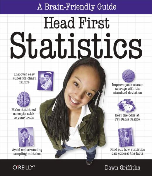
Wouldn't it be great if there were a statistics book that made histograms, probability distributions, and chi square analysis more enjoyable than going to the dentist? Head First Statistics brings this typically dry subject to life, teaching you everything you want and need to know about statistics through engaging, interactive, and thought-provoking material, full of puzzles, stories, quizzes, visual aids, and real-world examples.
Whether you're a student, a professional, or just curious about statistical analysis, Head First's brain-friendly formula helps you get a firm grasp of…mehr
Andere Kunden interessierten sich auch für
- Alex ReinhartStatistics Done Wrong17,99 €
- Geoffrey McLachlanThe Em Algorithm and Extensions181,99 €
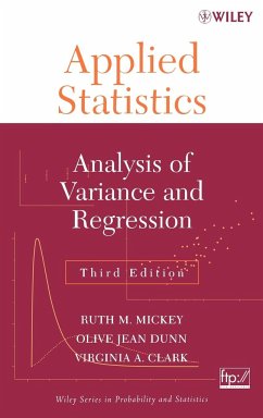
- Ruth M. MickeyApplied Statistics209,99 €
- Zehua ChenRanked Set Sampling83,99 €
- Marilyn K. PelosiElementary Statistics310,99 €
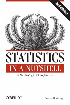
- Sarah BoslaughStatistics in a Nutshell47,99 €
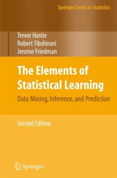
- Trevor HastieThe Elements of Statistical Learning68,99 €
-
-
-
Wouldn't it be great if there were a statistics book that made histograms, probability distributions, and chi square analysis more enjoyable than going to the dentist? Head First Statistics brings this typically dry subject to life, teaching you everything you want and need to know about statistics through engaging, interactive, and thought-provoking material, full of puzzles, stories, quizzes, visual aids, and real-world examples.
Whether you're a student, a professional, or just curious about statistical analysis, Head First's brain-friendly formula helps you get a firm grasp of statistics so you can understand key points and actually use them. Learn to present data visually with charts and plots; discover the difference between taking the average with mean, median, and mode, and why it's important; learn how to calculate probability and expectation; and much more.
Head First Statistics is ideal for high school and college students taking statistics and satisfies the requirements for passing the College Board's Advanced Placement (AP) Statistics Exam. With this book, you'll:
Study the full range of topics covered in first-year statistics
Tackle tough statistical concepts using Head First's dynamic, visually rich format proven to stimulate learning and help you retain knowledge
Explore real-world scenarios, ranging from casino gambling to prescription drug testing, to bring statistical principles to life
Discover how to measure spread, calculate odds through probability, and understand the normal, binomial, geometric, and Poisson distributions
Conduct sampling, use correlation and regression, do hypothesis testing, perform chi square analysis, and more
Before you know it, you'll not only have mastered statistics, you'll also see how they work in the real world. Head First Statistics will help you pass your statistics course, and give you a firm understanding of the subject so you can apply the knowledge throughout your life.
Hinweis: Dieser Artikel kann nur an eine deutsche Lieferadresse ausgeliefert werden.
Whether you're a student, a professional, or just curious about statistical analysis, Head First's brain-friendly formula helps you get a firm grasp of statistics so you can understand key points and actually use them. Learn to present data visually with charts and plots; discover the difference between taking the average with mean, median, and mode, and why it's important; learn how to calculate probability and expectation; and much more.
Head First Statistics is ideal for high school and college students taking statistics and satisfies the requirements for passing the College Board's Advanced Placement (AP) Statistics Exam. With this book, you'll:
Study the full range of topics covered in first-year statistics
Tackle tough statistical concepts using Head First's dynamic, visually rich format proven to stimulate learning and help you retain knowledge
Explore real-world scenarios, ranging from casino gambling to prescription drug testing, to bring statistical principles to life
Discover how to measure spread, calculate odds through probability, and understand the normal, binomial, geometric, and Poisson distributions
Conduct sampling, use correlation and regression, do hypothesis testing, perform chi square analysis, and more
Before you know it, you'll not only have mastered statistics, you'll also see how they work in the real world. Head First Statistics will help you pass your statistics course, and give you a firm understanding of the subject so you can apply the knowledge throughout your life.
Hinweis: Dieser Artikel kann nur an eine deutsche Lieferadresse ausgeliefert werden.
Produktdetails
- Produktdetails
- Verlag: O'Reilly Media
- Seitenzahl: 716
- Erscheinungstermin: September 2008
- Englisch
- Abmessung: 236mm x 205mm x 44mm
- Gewicht: 1038g
- ISBN-13: 9780596527587
- ISBN-10: 0596527586
- Artikelnr.: 23512498
- Herstellerkennzeichnung
- Libri GmbH
- Europaallee 1
- 36244 Bad Hersfeld
- 06621 890
- Verlag: O'Reilly Media
- Seitenzahl: 716
- Erscheinungstermin: September 2008
- Englisch
- Abmessung: 236mm x 205mm x 44mm
- Gewicht: 1038g
- ISBN-13: 9780596527587
- ISBN-10: 0596527586
- Artikelnr.: 23512498
- Herstellerkennzeichnung
- Libri GmbH
- Europaallee 1
- 36244 Bad Hersfeld
- 06621 890
Dawn Griffiths started life as a mathematician at a top UK university. She was awarded a First-Class Honours degree in Mathematics, and was offered a university scholarship to undertake a PhD studying particularly rare breeds of differential equations. She moved away from academia when she realized that people would stop talking to her at parties, and went on to pursue a career in software development instead. She currently combines IT consultancy with writing and mathematics. When Dawn's not working on Head First books, you'll find her honing her Tai Chi skills, making bobbin lace or cooking nice meals. She hasn't yet mastered the art of doing all three at the same time. She also enjoys traveling, and spending time with her lovely husband, David.
; Advance Praise for Head First Statistics; Praise for other Head First books; Author of Head First Statistics; How to use this Book: Intro; Who is this book for?; We know what you're thinking; We know what your brain is thinking; Metacognition: thinking about thinking; Here's what WE did; Read Me; The technical review team; Acknowledgments; Safari® Books Online; Chapter 1: Visualizing Information: First Impressions; 1.1 Statistics are everywhere; 1.2 But why learn statistics?; 1.3 A tale of two charts; 1.4 Manic Mango needs some charts; 1.5 The humble pie chart; 1.6 Chart failure; 1.7 Bar charts can allow for more accuracy; 1.8 Vertical bar charts; 1.9 Horizontal bar charts; 1.10 It's a matter of scale; 1.11 Using frequency scales; 1.12 Dealing with multiple sets of data; 1.13 Your bar charts rock; 1.14 Categories vs. numbers; 1.15 Dealing with grouped data; 1.16 To make a histogram, start by finding bar widths; 1.17 Manic Mango needs another chart; 1.18 Make the area of histogram bars proportional to frequency; 1.19 Step 1: Find the bar widths; 1.20 Step 2: Find the bar heights; 1.21 Step 3: Draw your chart-a histogram; 1.22 Histograms can't do everything; 1.23 Introducing cumulative frequency; 1.24 Drawing the cumulative frequency graph; 1.25 Choosing the right chart; 1.26 Manic Mango conquered the games market!; Chapter 2: Measuring Central Tendency: The Middle Way; 2.1 Welcome to the Health Club; 2.2 A common measure of average is the mean; 2.3 Mean math; 2.4 Dealing with unknowns; 2.5 Back to the mean; 2.6 Handling frequencies; 2.7 Back to the Health Club; 2.8 Everybody was Kung Fu fighting; 2.9 Our data has outliers; 2.10 The butler outliers did it; 2.11 Watercooler conversation; 2.12 Finding the median; 2.13 Business is booming; 2.14 The Little Ducklings swimming class; 2.15 Frequency Magnets; 2.16 Frequency Magnets; 2.17 What went wrong with the mean and median?; 2.18 Introducing the mode; 2.19 Congratulations!; Chapter 3: Measuring Variability and Spread: Power Ranges; 3.1 Wanted: one player; 3.2 We need to compare player scores; 3.3 Use the range to differentiate between data sets; 3.4 The problem with outliers; 3.5 We need to get away from outliers; 3.6 Quartiles come to the rescue; 3.7 The interquartile range excludes outliers; 3.8 Quartile anatomy; 3.9 We're not just limited to quartiles; 3.10 So what are percentiles?; 3.11 Box and whisker plots let you visualize ranges; 3.12 Variability is more than just spread; 3.13 Calculating average distances; 3.14 We can calculate variation with the variance...; 3.15 ...but standard deviation is a more intuitive measure; 3.16 A quicker calculation for variance; 3.17 What if we need a baseline for comparison?; 3.18 Use standard scores to compare values across data sets; 3.19 Interpreting standard scores; 3.20 Statsville All Stars win the league!; Chapter 4: Calculating Probabilities: Taking Chances; 4.1 Fat Dan's Grand Slam; 4.2 Roll up for roulette!; 4.3 Your very own roulette board; 4.4 Place your bets now!; 4.5 What are the chances?; 4.6 Find roulette probabilities; 4.7 You can visualize probabilities with a Venn diagram; 4.8 It's time to play!; 4.9 And the winning number is...; 4.10 Let's bet on an even more likely event; 4.11 You can also add probabilities; 4.12 You win!; 4.13 Time for another bet; 4.14 Exclusive events and intersecting events; 4.15 Problems at the intersection; 4.16 Some more notation; 4.17 Another unlucky spin...; 4.18 ...but it's time for another bet; 4.19 Conditions apply; 4.20 Find conditional probabilities; 4.21 You can visualize conditional probabilities with a probability tree; 4.22 Trees also help you calculate conditional probabilities; 4.23 Bad luck!; 4.24 We can find P(Black l Even) using the probabilities we already have; 4.25 Step 1: Finding P(Black n Even); 4.26 So where does this get us?; 4.27 Step 2: Finding P(Even); 4.28 Step 3: Finding P(Black l Even); 4.29 These results can be generalized to other problems; 4.30 Use the Law of Total Probability to find P(B); 4.31 Introducing Bayes' Theorem; 4.32 We have a winner!; 4.33 It's time for one last bet; 4.34 If events affect each other, they are dependent; 4.35 If events do not affect each other, they are independent; 4.36 More on calculating probability for independent events; 4.37 Winner! Winner!; Chapter 5: Using Discrete Probability Distributions: Manage Your Expectations; 5.1 Back at Fat Dan's Casino; 5.2 We can compose a probability distribution for the slot machine; 5.3 Expectation gives you a prediction of the results...; 5.4 ... and variance tells you about the spread of the results; 5.5 Variances and probability distributions; 5.6 Let's calculate the slot machine's variance; 5.7 Fat Dan changed his prices; 5.8 There's a linear relationship between E(X) and E(Y); 5.9 Slot machine transformations; 5.10 General formulas for linear transforms; 5.11 Every pull of the lever is an independent observation; 5.12 Observation shortcuts; 5.13 New slot machine on the block; 5.14 Add E(X) and E(Y) to get E(X + Y)...; 5.15 ... and subtract E(X) and E(Y) to get E(X - Y); 5.16 You can also add and subtract linear transformations; 5.17 Jackpot!; Chapter 6: Permutations and Combinations: Making Arrangements; 6.1 The Statsville Derby; 6.2 It's a three-horse race; 6.3 How many ways can they cross the finish line?; 6.4 Calculate the number of arrangements; 6.5 Going round in circles; 6.6 It's time for the novelty race; 6.7 Arranging by individuals is different than arranging by type; 6.8 We need to arrange animals by type; 6.9 Generalize a formula for arranging duplicates; 6.10 It's time for the twenty-horse race; 6.11 How many ways can we fill the top three positions?; 6.12 Examining permutations; 6.13 What if horse order doesn't matter; 6.14 Examining combinations; 6.15 It's the end of the race; Chapter 7: Geometric, Binomial, and Poisson Distributions: Keeping Things Discrete; 7.1 Meet Chad, the hapless snowboarder; 7.2 We need to find Chad's probability distribution; 7.3 There's a pattern to this probability distribution; 7.4 The probability distribution can be represented algebraically; 7.5 The pattern of expectations for the geometric distribution; 7.6 Expectation is 1/p; 7.7 Finding the variance for our distribution; 7.8 You've mastered the geometric distribution; 7.9 Should you play, or walk away?; 7.10 Generalizing the probability for three questions; 7.11 Let's generalize the probability further; 7.12 What's the expectation and variance?; 7.13 Binomial expectation and variance; 7.14 The Statsville Cinema has a problem; 7.15 Expectation and variance for the Poisson distribution; 7.16 So what's the probability distribution?; 7.17 Combine Poisson variables; 7.18 The Poisson in disguise; 7.19 Anyone for popcorn?; Chapter 8: Using the Normal Distribution: Being Normal; 8.1 Discrete data takes exact values...; 8.2 ... but not all numeric data is discrete; 8.3 What's the delay?; 8.4 We need a probability distribution for continuous data; 8.5 Probability density functions can be used for continuous data; 8.6 Probability = area; 8.7 To calculate probability, start by finding f(x)...; 8.8 ... then find probability by finding the area; 8.9 We've found the probability; 8.10 Searching for a soul sole mate; 8.11 Male modelling; 8.12 The normal distribution is an "ideal" model for continuous data; 8.13 So how do we find normal probabilities?; 8.14 Three steps to calculating normal probabilities; 8.15 Step 1: Determine your distribution; 8.16 Step 2: Standardize to N(0, 1); 8.17 To standardize, first move the mean...; 8.18 ... then squash the width; 8.19 Now find Z for the specific value you want to find probability for; 8.20 Step 3: Look up the probability in your handy table; 8.21 Julie's probability is in the table; 8.22 And they all lived happily ever after; Chapter 9: Using the Normal Distribution ii: Beyond Normal; 9.1 Love is a roller coaster; 9.2 All aboard the Love Train; 9.3 Normal bride + normal groom; 9.4 It's still just weight; 9.5 How's the combined weight distributed?; 9.6 Finding probabilities; 9.7 More people want the Love Train; 9.8 Linear transforms describe underlying changes in values...; 9.9 ...and independent observations describe how many values you have; 9.10 Expectation and variance for independent observations; 9.11 Should we play, or walk away?; 9.12 Normal distribution to the rescue; 9.13 When to approximate the binomial distribution with the normal; 9.14 Revisiting the normal approximation; 9.15 The binomial is discrete, but the normal is continuous; 9.16 Apply a continuity correction before calculating the approximation; 9.17 All aboard the Love Train; 9.18 When to approximate the binomial distribution with the normal; 9.19 A runaway success!; Chapter 10: Using Statistical Sampling: Taking Samples; 10.1 The Mighty Gumball taste test; 10.2 They're running out of gumballs; 10.3 Test a gumball sample, not the whole gumball population; 10.4 How sampling works; 10.5 When sampling goes wrong; 10.6 How to design a sample; 10.7 Define your sampling frame; 10.8 Sometimes samples can be biased; 10.9 Sources of bias; 10.10 How to choose your sample; 10.11 Simple random sampling; 10.12 How to choose a simple random sample; 10.13 There are other types of sampling; 10.14 We can use stratified sampling...; 10.15 ...or we can use cluster sampling...; 10.16 ...or even systematic sampling; 10.17 Mighty Gumball has a sample; Chapter 11: Estimating Populations and Samples: Making Predictions; 11.1 So how long does flavor really last for?; 11.2 Let's start by estimating the population mean; 11.3 Point estimators can approximate population parameters; 11.4 Let's estimate the population variance; 11.5 We need a different point estimator than sample variance; 11.6 Which formula's which?; 11.7 Mighty Gumball has done more sampling; 11.8 It's a question of proportion; 11.9 Buy your gumballs here!; 11.10 So how does this relate to sampling?; 11.11 The sampling distribution of proportions; 11.12 So what's the expectation of Ps?; 11.13 And what's the variance of Ps?; 11.14 Find the distribution of Ps; 11.15 Ps follows a normal distribution; 11.16 How many gumballs?; 11.17 We need probabilities for the sample mean; 11.18 The sampling distribution of the mean; 11.19 Find the expectation for X¯; 11.20 What about the the variance of X¯?; 11.21 So how is X¯ distributed?; 11.22 If n is large, X¯ can still be approximated by the normal distribution; 11.23 Using the central limit theorem; 11.24 Sampling saves the day!; Chapter 12: Constructing Confidence Intervals: Guessing with Confidence; 12.1 Mighty Gumball is in trouble; 12.2 The problem with precision; 12.3 Introducing confidence intervals; 12.4 Four steps for finding confidence intervals; 12.5 Step 1: Choose your population statistic; 12.6 Step 2: Find its sampling distribution; 12.7 Point estimators to the rescue; 12.8 We've found the distribution for X¯; 12.9 Step 3: Decide on the level of confidence; 12.10 How to select an appropriate confidence level; 12.11 Step 4: Find the confidence limits; 12.12 Start by finding Z; 12.13 Rewrite the inequality in terms of µ; 12.14 Finally, find the value of X¯; 12.15 You've found the confidence interval; 12.16 Let's summarize the steps; 12.17 Handy shortcuts for confidence intervals; 12.18 Just one more problem...; 12.19 Step 1: Choose your population statistic; 12.20 Step 2: Find its sampling distribution; 12.21 X¯ follows the t-distribution when the sample is small; 12.22 Find the standard score for the t-distribution; 12.23 Step 3: Decide on the level of confidence; 12.24 Step 4: Find the confidence limits; 12.25 Using t-distribution probability tables; 12.26 The t-distribution vs. the normal distribution; 12.27 You've found the confidence intervals!; Chapter 13: Using Hypothesis Tests: Look At The Evidence; 13.1 Statsville's new miracle drug; 13.2 So what's the problem?; 13.3 Resolving the conflict from 50,000 feet; 13.4 The six steps for hypothesis testing; 13.5 Step 1: Decide on the hypothesis; 13.6 So what's the alternative?; 13.7 Step 2: Choose your test statistic; 13.8 Step 3: Determine the critical region; 13.9 To find the critical region, first decide on the significance level; 13.10 Step 4: Find the p-value; 13.11 We've found the p-value; 13.12 Step 5: Is the sample result in the critical region?; 13.13 Step 6: Make your decision; 13.14 So what did we just do?; 13.15 What if the sample size is larger?; 13.16 Let's conduct another hypothesis test; 13.17 Step 1: Decide on the hypotheses; 13.18 Step 2: Choose the test statistic; 13.19 Use the normal to approximate the binomial in our test statistic; 13.20 Step 3: Find the critical region; 13.21 SnoreCull failed the test; 13.22 Mistakes can happen; 13.23 Let's start with Type I errors; 13.24 What about Type II errors?; 13.25 Finding errors for SnoreCull; 13.26 We need to find the range of values; 13.27 Find P(Type II error); 13.28 Introducing power; 13.29 The doctor's happy; Chapter 14: The
2 Distribution: There's Something Going On...; 14.1 There may be trouble ahead at Fat Dan's Casino; 14.2 Let's start with the slot machines; 14.3 The
2 test assesses difference; 14.4 So what does the test statistic represent?; 14.5 Two main uses of the
2 distribution; 14.6 v represents degrees of freedom; 14.7 What's the significance?; 14.8 Hypothesis testing with
2; 14.9 You've solved the slot machine mystery; 14.10 Fat Dan has another problem; 14.11 the
2 distribution can test for independence; 14.12 You can find the expected frequencies using probability; 14.13 So what are the frequencies?; 14.14 We still need to calculate degrees of freedom; 14.15 Generalizing the degrees of freedom; 14.16 And the formula is...; 14.17 You've saved the casino; Chapter 15: Correlation and Regression: What's My Line?; 15.1 Never trust the weather; 15.2 Let's analyze sunshine and attendance; 15.3 Exploring types of data; 15.4 Visualizing bivariate data; 15.5 Scatter diagrams show you patterns; 15.6 Correlation vs. causation; 15.7 Predict values with a line of best fit; 15.8 Your best guess is still a guess; 15.9 We need to minimize the errors; 15.10 Introducing the sum of squared errors; 15.11 Find the equation for the line of best fit; 15.12 Finding the slope for the line of best fit; 15.13 Finding the slope for the line of best fit, part ii; 15.14 We've found b, but what about a?; 15.15 You've made the connection; 15.16 Let's look at some correlations; 15.17 The correlation coefficient measures how well the line fits the data; 15.18 There's a formula for calculating the correlation coefficient, r; 15.19 Find r for the concert data; 15.20 Find r for the concert data, continued; 15.21 You've saved the day!; 15.22 Leaving town...; 15.23 It's been great having you here in Statsville!; Leftovers: The Top Ten Things (we didn't cover); #1. Other ways of presenting data; #2. Distribution anatomy; #3. Experiments; Designing your experiment; #4. Least square regression alternate notation; #5. The coefficient of determination; #6. Non-linear relationships; #7. The confidence interval for the slope of a regression line; #8. Sampling distributions - the difference between two means; #9. Sampling distributions - the difference between two proportions; #10. E(X) and Var(X) for continuous probability distributions; Finding E(X); Finding Var(X); Statistics Tables: Looking Things Up; #1. Standard normal probabilities; #2. t-distribution critical values; #3. X2 critical values;