N. W. Galwey

Introduction to Mixed Modelling

Beyond Regression and Analysis of Variance

• Gebundenes Buch

Produktbeschreibung

Mixed modelling is very useful, and easier than you think!
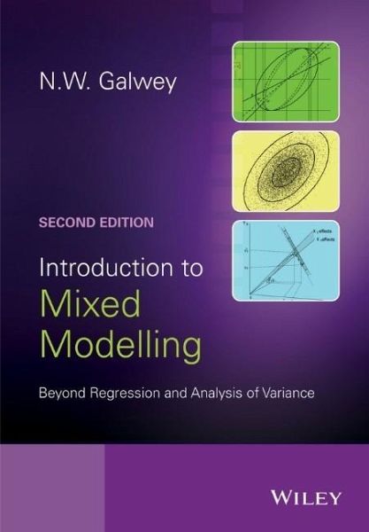
Mixed modelling is now well established as a powerful approach to statistical data analysis. It is based on the recognition of random-effect terms in statistical models, leading to inferences and estimates that have much wider applicability and are more realistic than those otherwise obtained.
Introduction to Mixed Modelling leads the reader into mixed modelling as a natural extension of two more familiar methods, regression analysis and analysis of variance. It provides practical guidance combined with a clear explanation of the underlying concepts.
Like the first edition, this new edition shows diverse applications of mixed models, provides guidance on the identification of random-effect terms, and explains how to obtain and interpret best linear unbiased predictors (BLUPs). It also introduces several important new topics, including the following:
Use of the software SAS, in addition to GenStat and R.
Meta-analysis and the multiple testing problem.
The Bayesian interpretation of mixed models.
Including numerous practical exercises with solutions, this book provides an ideal introduction to mixed modelling for final year undergraduate students, postgraduate students and professional researchers. It will appeal to readers from a wide range of scientific disciplines including statistics, biology, bioinformatics, medicine, agriculture, engineering, economics, archaeology and geography.
Praise for the first edition:
"One of the main strengths of the text is the bridge it provides between traditional analysis of variance and regression models and the more recently developed class of mixed models...Each chapter is well-motivated by at least one carefully chosen example...demonstrating the broad applicability of mixed models in many different disciplines...most readers will likely learn something new, and those previously unfamiliar with mixed models will obtain a solid foundation on this topic."- Kerrie Nelson University of South Carolina, in American Statistician, 2007

---

Hinweis: Dieser Artikel kann nur an eine deutsche Lieferadresse ausgeliefert werden.

Produktdetails

• Verlag: Wiley & Sons
• Artikelnr. des Verlages: 1W119945490
• 2. Aufl.
• Seitenzahl: 504
• Erscheinungstermin: 10. November 2014
• Englisch
• Abmessung: 251mm x 174mm x 32mm
• Gewicht: 907g
• ISBN-13: 9781119945499
• ISBN-10: 1119945496
• Artikelnr.: 40553161

Autorenporträt

Nicholas W. Galwey, Statistical Consultant, GlaxoSmithKline, Harlow, Essex, UK.

Inhaltsangabe

Preface xi
1 The need for more than one random-effect term when fitting a regression
line 1
1.1 A data set with several observations of variable Y at each value of
variable X 1
1.2 Simple regression analysis: Use of the software GenStat to perform the
analysis 2
1.3 Regression analysis on the group means 9
1.4 A regression model with a term for the groups 10
1.5 Construction of the appropriate F test for the significance of the
explanatory variable when groups are present 13
1.6 The decision to specify a model term as random: A mixed model 14
1.7 Comparison of the tests in a mixed model with a test of lack of fit 16
1.8 The use of REsidual Maximum Likelihood (REML) to fit the mixed model 17
1.9 Equivalence of the different analyses when the number of observations
per group is constant 21
1.10 Testing the assumptions of the analyses: Inspection of the residual
values 26
1.11 Use of the software R to perform the analyses 28
1.12 Use of the software SAS to perform the analyses 33
1.13 Fitting a mixed model using GenStat's Graphical User Interface (GUI)
40
1.14 Summary 46
1.15 Exercises 47
References 51
2 The need for more than one random-effect term in a designed experiment 52
2.1 The split plot design: A design with more than one random-effect term
52
2.2 The analysis of variance of the split plot design: A random-effect term
for the main plots 54
2.3 Consequences of failure to recognize the main plots when analysing the
split plot design 62
2.4 The use of mixed modelling to analyse the split plot design 64
2.5 A more conservative alternative to the F and Wald statistics 66
2.6 Justification for regarding block effects as random 67
2.7 Testing the assumptions of the analyses: Inspection of the residual
values 68
2.8 Use of R to perform the analyses 71
2.9 Use of SAS to perform the analyses 77
2.10 Summary 81
2.11 Exercises 82
References 86
3 Estimation of the variances of random-effect terms 87
3.1 The need to estimate variance components 87
3.2 A hierarchical random-effects model for a three-stage assay process 87
3.3 The relationship between variance components and stratum mean squares
91
3.4 Estimation of the variance components in the hierarchical
random-effects model 93
3.5 Design of an optimum strategy for future sampling 95
3.6 Use of R to analyse the hierarchical three-stage assay process 98
3.7 Use of SAS to analyse the hierarchical three-stage assay process 100
3.8 Genetic variation: A crop field trial with an unbalanced design 102
3.9 Production of a balanced experimental design by 'padding' with missing
values 106
3.10 Specification of a treatment term as a random-effect term: The use of
mixed-model analysis to analyse an unbalanced data set 110
3.11 Comparison of a variance component estimate with its standard error
112
3.12 An alternative significance test for variance components 113
3.13 Comparison among significance tests for variance components 116
3.14 Inspection of the residual values 117
3.15 Heritability: The prediction of genetic advance under selection 117
3.16 Use of R to analyse the unbalanced field trial 122
3.17 Use of SAS to analyse the unbalanced field trial 125
3.18 Estimation of variance components in the regression analysis on
grouped data 128
3.19 Estimation of variance components for block effects in the split-plot
experimental design 130
3.20 Summary 132
3.21 Exercises 133
References 136
4 Interval estimates for fixed-effect terms in mixed models 137
4.1 The concept of an interval estimate 137
4.2 Standard errors for regression coefficients in a mixed-model analysis
138
4.3 Standard errors for differences between treatment means in the
split-plot design 142
4.4 A significance test for the difference between treatment means 144
4.5 The least significant difference (LSD) between treatment means 147
4.6 Standard errors for treatment means in designed experiments: A
difference in approach between analysis of variance and mixed-model
analysis 151
4.7 Use of R to obtain SEs of means in a designed experiment 157
4.8 Use of SAS to obtain SEs of means in a designed experiment 159
4.9 Summary 161
4.10 Exercises 163
References 164
5 Estimation of random effects in mixed models: Best Linear Unbiased
Predictors (BLUPs) 165
5.1 The difference between the estimates of fixed and random effects 165
5.2 The method for estimation of random effects: The best linear unbiased
predictor (BLUP) or 'shrunk estimate' 168
5.3 The relationship between the shrinkage of BLUPs and regression towards
the mean 170
5.4 Use of R for the estimation of fixed and random effects 176
5.5 Use of SAS for the estimation of random effects 178
5.6 The Bayesian interpretation of BLUPs: Justification of a random-effect
term without invoking an underlying infinite population 182
5.7 Summary 187
5.8 Exercises 188
References 191
6 More advanced mixed models for more elaborate data sets 192
6.1 Features of the models introduced so far: A review 192
6.2 Further combinations of model features 192
6.3 The choice of model terms to be specified as random 195
6.4 Disagreement concerning the appropriate significance test when fixed
and random-effect terms interact: 'The great mixed-model muddle' 197
6.5 Arguments for specifying block effects as random 204
6.6 Examples of the choice of fixed- and random-effect specification of
terms 209
6.7 Summary 213
6.8 Exercises 215
References 216
7 Three case studies 217
7.1 Further development of mixed modelling concepts through the analysis of
specific data sets 217
7.2 A fixed-effects model with several variates and factors 218
7.3 Use of R to fit the fixed-effects model with several variates and
factors 233
7.4 Use of SAS to fit the fixed-effects model with several variates and
factors 237
7.5 A random coefficient regression model 242
7.6 Use of R to fit the random coefficients model 246
7.7 Use of SAS to fit the random coefficients model 247
7.8 A random-effects model with several factors 249
7.9 Use of R to fit the random-effects model with several factors 266
7.10 Use of SAS to fit the random-effects model with several factors 274
7.11 Summary 282
7.12 Exercises 282
References 294
8 Meta-analysis and the multiple testing problem 295
8.1 Meta-analysis: Combined analysis of a set of studies 295
8.2 Fixed-effect meta-analysis with estimation only of the main effect of
treatment 296
8.3 Random-effects meta-analysis with estimation of study × treatment
interaction effects 301
8.4 A random-effect interaction between two fixed-effect terms 303
8.5 Meta-analysis of individual-subject data using R 307
8.6 Meta-analysis of individual-subject data using SAS 312
8.7 Meta-analysis when only summary data are available 318
8.8 The multiple testing problem: Shrinkage of BLUPs as a defence against
the Winner's Curse 326
8.9 Fitting of multiple models using R 338
8.10 Fitting of multiple models using SAS 340
8.11 Summary 342
8.12 Exercises 343
References 348
9 The use of mixed models for the analysis of unbalanced experimental
designs 350
9.1 A balanced incomplete block design 350
9.2 Imbalance due to a missing block: Mixed-model analysis of the
incomplete block design 354
9.3 Use of R to analyse the incomplete block design 358
9.4 Use of SAS to analyse the incomplete block design 360
9.5 Relaxation of the requirement for balance: Alpha designs 362
9.6 Approximate balance in two directions: The alphalpha design 368
9.7 Use of R to analyse the alphalpha design 373
9.8 Use of SAS to analyse the alphalpha design 374
9.9 Summary 376
9.10 Exercises 377
References 378
10 Beyond mixed modelling 379
10.1 Review of the uses of mixed models 379
10.2 The generalized linear mixed model (GLMM): Fitting a logistic
(sigmoidal) curve to proportions of observations 380
10.3 Use of R to fit the logistic curve 388
10.4 Use of SAS to fit the logistic curve 390
10.5 Fitting a GLMM to a contingency table: Trouble-shooting when the mixed
modelling process fails 392
10.6 The hierarchical generalized linear model (HGLM) 403
10.7 Use of R to fit a GLMM and a HGLM to a contingency table 410
10.8 Use of SAS to fit a GLMM to a contingency table 415
10.9 The role of the covariance matrix in the specification of a mixed
model 418
10.10 A more general pattern in the covariance matrix: Analysis of
pedigrees and genetic data 421
10.11 Estimation of parameters in the covariance matrix: Analysis of
temporal and spatial variation 431
10.12 Use of R to model spatial variation 441
10.13 Use of SAS to model spatial variation 444
10.14 Summary 447
10.15 Exercises 447
References 452
11 Why is the criterion for fitting mixed models called REsidual Maximum
Likelihood? 454
11.1 Maximum likelihood and residual maximum likelihood 454
11.2 Estimation of the variance 2 from a single observation using the
maximum-likelihood criterion 455
11.3 Estimation of 2 from more than one observation 455
11.4 The -effect axis as a dimension within the sample space 457
11.5 Simultaneous estimation of and 2 using the maximum-likelihood
criterion 460
11.6 An alternative estimate of 2 using the REML criterion 462
11.7 Bayesian justification of the REML criterion 465
11.8 Extension to the general linear model: The fixed-effect axes as a
sub-space of the sample space 465
11.9 Application of the REML criterion to the general linear model 470
11.10 Extension to models with more than one random-effect term 472
11.11 Summary 473
11.12 Exercises 474
References 476
Index 477