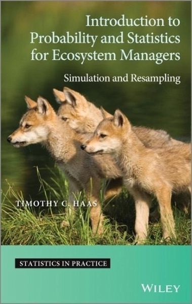
Timothy C. Haas

Introduction to Probability and Statistics for Ecosystem Managers

Simulation and Resampling

• Gebundenes Buch

Produktbeschreibung

Explores computer-intensive probability and statistics for ecosystem management decision making

Simulation is an accessible way to explain probability and stochastic model behavior to beginners. This book introduces probability and statistics to future and practicing ecosystem managers by providing a comprehensive treatment of these two areas. The author presents a self-contained introduction for individuals involved in monitoring, assessing, and managing ecosystems and features intuitive, simulation-based explanations of probabilistic and statistical concepts. Mathematical programming details are provided for estimating ecosystem model parameters with Minimum Distance, a robust and computer-intensive method.

The majority of examples illustrate how probability and statistics can be applied to ecosystem management challenges. There are over 50 exercises - making this book suitable for a lecture course in a natural resource and/or wildlife management department, or as the main text in a program of self-study.

Key features:
Reviews different approaches to wildlife and ecosystem management and inference.
Uses simulation as an accessible way to explain probability and stochastic model behavior to beginners.
Covers material from basic probability through to hierarchical Bayesian models and spatial/ spatio-temporal statistical inference.
Provides detailed instructions for using R, along with complete R programs to recreate the output of the many examples presented.
Provides an introduction to Geographic Information Systems (GIS) along with examples from Quantum GIS, a free GIS software package.
A companion website featuring all R code and data used throughout the book.
Solutions to all exercises are presented along with an online intelligent tutoring system that supports readers who are using the book for self-study.

---

Hinweis: Dieser Artikel kann nur an eine deutsche Lieferadresse ausgeliefert werden.

Produktdetails

• Statistics in Practice .1
• Verlag: Wiley & Sons
• 1. Auflage
• Seitenzahl: 312
• Erscheinungstermin: 29. Juli 2013
• Englisch
• Abmessung: 231mm x 157mm x 20mm
• Gewicht: 556g
• ISBN-13: 9781118357682
• ISBN-10: 111835768X
• Artikelnr.: 38133431

Autorenporträt

Timothy C. Haas, Lubar School of Business Administration, University of Wisconsin at Milwaukee. Timothy Haas is involved in teaching undergraduate and graduate courses in statistical methods, pursuing decision making and environmental statistics re?search, and collaborating with faculty on application of statistics to Marketing and Eco?nomics.

Inhaltsangabe

List of figures xiii List of tables xvii Preface xix Acknowledgments xxi List of abbreviations xxiii 1 Introduction 1 1.1 The textbook's purpose 1 1.1.1 The textbook's focus on ecosystem management 2 1.1.2 Reader level, prerequisites, and typical reader jobs 3 1.2 The textbook's pedagogical approach 4 1.2.1 General points 4 1.2.2 Use of this textbook for self-study 4 1.2.3 Learning resources 5 1.3 Chapter summaries 7 1.4 Installing and running R Commander 9 1.4.1 Running R 9 1.4.2 Starting an R Commander session 9 1.4.3 Terminating an R Commander session 10 1.5 Introductory R Commander session 10 1.6 Teaching probability through simulation 13 1.6.1 The frequentist statistical inference paradigm 14 1.7 Summary 15 2 Probability and simulation 17 2.1 Introduction 17 2.2 Basic probability 17 2.2.1 Definitions 17 2.2.2 Independence 20 2.3 Random variables 22 2.3.1 Definitions 22 2.3.2 Simulating random variables 26 2.3.3 A random variable's expected value (mean) and variance 26 2.3.4 Details of the normal (Gaussian) distribution 28 2.3.5 Distribution approximations 30 2.4 Joint distributions 31 2.4.1 Definition 31 2.4.2 Mixed variables 32 2.4.3 Marginal distribution 32 2.4.4 Conditional distributions 33 2.4.5 Independent random variables 34 2.5 Influence diagrams 34 2.5.1 Definitions 34 2.5.2 Example of a Bayesian network in ecosystem management 36 2.5.3 Modeling causal relationships with an influence diagram 38 2.6 Advantages of influence diagrams in ecosystem management 40 2.7 Two ecosystem management Bayesian networks 41 2.7.1 Waterbody eutrophication 41 2.7.2 Wildlife population viability 41 2.8 Influence diagram sensitivity analysis 41 2.9 Drawbacks to influence diagrams 42 3 Application of probability: Models of political decision making in ecosystem management 43 3.1 Introduction 43 3.2 Influence diagram models of decision making 43 3.2.1 Ecosystem status perception nodes 44 3.2.2 Image nodes 44 3.2.3 Economic, militaristic, and institutional goal nodes 45 3.2.4 Audience effect nodes 45 3.2.5 Resource nodes 46 3.2.6 Action and target nodes 46 3.2.7 Overall goal attainment node 47 3.2.8 How a group influence diagram reaches a decision 47 3.2.9 An advantage of this decision-making architecture 47 3.2.10 Evaluation dimensions 47 3.3 Rhino poachers: A simplified model 50 3.4 Policymakers: A simplified model 57 3.5 Conclusions 59 4 Statistical inference I: Basic ideas and parameter estimation 61 4.1 Definitions of some fundamental terms 61 4.2 Estimating the PDF and CDF 62 4.2.1 Histograms 62 4.2.2 Ogive 64 4.3 Measures of central tendency and dispersion 64 4.4 Sample quantiles 65 4.4.1 Sample quartiles 65 4.4.2 Sample deciles and percentiles 65 4.5 Distribution of a statistic 65 4.5.1 Basic setup in statistics 65 4.5.2 Sampling distributions 66 4.5.3 Normal quantile-quantile plot 66 4.6 The central limit theorem 68 4.7 Parameter estimation 68 4.7.1 Bias, variance, and efficiency 69 4.8 Interval estimates 70 4.8.1 A confidence interval for
when
2 is known 70 4.9 Basic regression analysis 71 4.9.1 Definitions and fundamental characteristics 71 4.9.2 The regression model 72 4.9.3 Correlation 74 4.9.4 Sampling distributions 75 4.9.5 Prediction and estimation 76 4.9.6 Misuse of regression models 76 4.10 General methods of parameter estimation 79 4.10.1 Maximum likelihood 79 4.10.2 Minimum Hellinger distance 80 4.10.3 Consistency analysis 80 5 Statistical inference II: Hypothesis tests 83 5.1 Introduction 83 5.2 Hypothesis tests: General definitions and properties 83 5.2.1 Definitions and procedure 83 5.2.2 Confidence intervals and hypothesis tests 85 5.2.3 Types of mistakes 85 5.2.4 One way to set the test's level 86 5.2.5 The z -test for hypotheses about
89 5.2.6 p-Values 91 5.3 Power 92 5.3.1 Power curves 93 5.4 t-Tests and a test for equal variances 95 5.4.1 The t -test 95 5.4.2 Two-sample t -tests 95 5.4.3 Tests for paired data 96 5.4.4 Testing for equal variances 98 5.5 Hypothesis tests on the regression model 98 5.5.1 Prediction and estimation confidence intervals 103 5.5.2 Multiple regression 104 5.5.3 Original scale prediction in regression 106 5.6 Brief introduction to vectors and matrices 106 5.6.1 Basic definitions 106 5.6.2 Inverse of a matrix 108 5.6.3 Random vectors and random matrices 108 5.7 Matrix form of multiple regression 109 5.7.1 Generalized least squares 111 5.8 Hypothesis testing with the delete-d jackknife 111 5.8.1 Background 111 5.8.2 A one-sample delete-d jackknife test 111 5.8.3 Testing classifier error rates 114 5.8.4 Important points about this test 115 5.8.5 Parameter confidence intervals 115 6 Introduction to spatial statistics 117 6.1 Overview 117 6.1.1 Types of spatial processes 118 6.2 Spatial statistics and GIS 118 6.2.1 Types of spatial data 118 6.3 QGIS 121 6.3.1 Capabilities 122 6.3.2 Installing QGIS 122 6.3.3 Documentation and tutorials 122 6.3.4 Installing plugins 123 6.3.5 How to convert a text file to a shapefile 123 6.4 Continuous spatial processes 125 6.4.1 Definitions 125 6.4.2 Graphical tools for exploring continuous spatial data 127 6.4.3 Third- and fourth-order cumulant minimization 132 6.4.4 Best linear unbiased predictor 132 6.4.5 Kriging variance 134 6.4.6 Model-fitting diagnostics 136 6.4.7 Kriging within a window 137 6.5 Spatial point processes 138 6.5.1 Definitions 138 6.5.2 Marked spatial point processes 149 6.5.3 Conclusions 150 6.6 Continuously valued multivariate processes 151 6.6.1 Fitting multivariate covariance functions 151 6.6.2 Cokriging: The MWRCK procedure 155 7 Introduction to spatio-temporal statistics 159 7.1 Introduction 159 7.2 Representing time in a GIS 159 7.2.1 The QGIS Time Manager plugin 160 7.2.2 A Clifford algebra-based spatio-temporal data structure 163 7.2.3 A raster- and event-based spatio-temporal data model 163 7.2.4 Application of ESTDM to a land cover study 166 7.3 Spatio-temporal prediction: MCSTK 166 7.3.1 Algorithms 166 7.3.2 Covariogram model and its estimator 169 7.4 Multivariate processes 174 7.4.1 Definitions 175 7.4.2 Transformations 175 7.4.3 Covariograms and cross-covariograms 180 7.4.4 Parameter estimation 181 7.4.5 Prediction algorithms 182 7.4.6 Cross-validation 183 7.4.7 Summary 190 7.5 Spatio-temporal point processes 190 7.6 Marked spatio-temporal point processes 195 7.6.1 A mark semivariogram estimator 196 8 Application of statistical inference: Estimating the parameters of an individual-based model 199 8.1 Overview 199 8.2 A simple IBM and its estimation 200 8.2.1 Simple IBM 200 8.2.2 Parameter estimation 201 8.3 Fitting IBMs with MSHD 204 8.3.1 Ergodicity 206 8.3.2 Observable random variables from IBM output 207 8.4 Further properties of parameter estimators 207 8.4.1 Consistency 207 8.4.2 Robustness 208 8.5 Parameter confidence intervals for a nonergodic model 209 8.6 Rhino-supporting ecosystem influence diagram 209 8.6.1 Spatial effects on poaching 210 8.6.2 IBM variables 213 8.6.3 Initial conditions and hypothesis values of parameters 214 8.6.4 Mapping functions 215 8.6.5 Realism of ecosystem influence diagram output 217 8.7 Estimation of rhino IBM parameters 219 8.7.1 Parameter confidence intervals 220 9 Guiding an influence diagram's learning 223 9.1 Introduction 223 9.2 Online learning of Bayesian network parameters 224 9.2.1 Basic algorithm using simulation 224 9.2.2 Updating influence diagrams 225 9.3 Learning an influence diagram's structure 229 9.3.1 Minimum description length score function 229 9.3.2 Description length of an edge 229 9.3.3 Random generation of DAGs 230 9.3.4 Algorithm to detect and delete cycles 230 9.3.5 Mutate functions 231 9.3.6 MDLEP algorithm 232 9.3.7 Using MDLEP to learn influence diagram structure 232 9.4 Feedback-based learning for group decision-making diagrams 233 9.4.1 Definitions and algorithm 233 9.5 Summary and conclusions 234 10 Fitting and testing a political-ecological simulator 235 10.1 Introduction 235 10.1.1 Background on rhino poaching 236 10.1.2 Scenarios wherein rhino poaching is reduced 237 10.2 EMT simulator construction 237 10.2.1 Modeled groups 237 10.2.2 Rhino-supporting ecosystem influence diagram 248 10.3 Consistency analysis estimates of simulator parameters 248 10.4 MPEMP computation 251 10.4.1 Setup 251 10.4.2 Solution 253 10.5 Conclusions 254 Appendix 257 Simpson's rule in two dimensions 257 References 263 Index 275