Johan Schoukens, Rik Pintelon, Yves Rolain

Mastering System Identification

• Broschiertes Buch

Produktbeschreibung

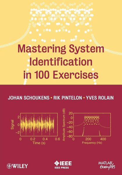
Systems identification is a general term used to describe mathematical tools and algorithms that build dynamical models from measured data. Mastering System Identification in 100 Exercises takes readers step by step through a series of MATLAB exercises that teach how to measure and model linear dynamic systems in the presence of nonlinear distortions from a practical point of view. Each exercise is followed by a short discussion illustrating what lessons can be learned by the reader.
The book, with its learn-by-doing approach, also includes:
State-of-the-art system identification methods, with both time and frequency domain system identification methods--including the pros and cons of each
Simple writing style with numerous examples and figures
Downloadable author-programmed MATLAB files for each exercise--with detailed solutions
Larger projects that serve as potential assignments
Covering both classic and recent measurement and identifying methods, this book will appeal to practicing engineers, scientists, and researchers, as well as master's and PhD students in electrical, mechanical, civil, and chemical engineering.

---

Hinweis: Dieser Artikel kann nur an eine deutsche Lieferadresse ausgeliefert werden.

Produktdetails

• Verlag: Wiley & Sons
• 1. Auflage
• Seitenzahl: 282
• Erscheinungstermin: 26. März 2012
• Englisch
• Abmessung: 254mm x 178mm x 16mm
• Gewicht: 666g
• ISBN-13: 9780470936986
• ISBN-10: 0470936983
• Artikelnr.: 34158786

Autorenporträt

Johan Schoukens, PhD, serves as a full-time professor in the ELEC Department at the Vrije Universiteit Brussel. He has been a Fellow of IEEE since 1997 and was the recipient of the 2003 IEEE Instrumentation and Measurement Society Distinguished Service Award. Rik Pintelon, PhD, serves as a full-time professor at the Vrije Universiteit Brussel in the ELEC Department. He has been a Fellow of IEEE since 1998 and is the recipient of the 2012 IEEE Joseph F. Keithley Award in Instrumentation and Measurement (IEEE Technical Field Award). Yves Rolain, PhD, serves as a full-time professor at the Vrije Universiteit Brussel in the ELEC department. He has been a Fellow of IEEE since 2006 and was the recipient of the 2004 IEEE Instrumentation and Measurement Society Technical Award.

Inhaltsangabe

Preface xiii
Acknowledgments xv
Abbreviations xvii
1 Identification 1
1.1 Introduction 1
1.2 Illustration of Some Important Aspects of System Identification 2
Exercise 1 .a (Least squares estimation of the value of a resistor) 2
Exercise 1 .b (Analysis of the standard deviation) 3
Exercise 2 (Study of the asymptotic distribution of an estimate) 5
Exercise 3 (Impact of noise on the regressor (input) measurements) 6
Exercise 4 (Importance of the choice of the independent variable or input)
7
Exercise 5.a (combining measurements with a varying SNR: Weighted least
squares estimation) 8
Exercise 5.b (Weighted least squares estimation: A study of the variance) 9
Exercise 6 (Least squares estimation of models that are linear in the
parameters) 11
Exercise 7 (Characterizing a 2-dimensional parameter estimate) 12
1.3 Maximum Likelihood Estimation for Gaussian and Laplace Distributed
Noise 14
Exercise 8 (Dependence of the optimal cost function on the distribution of
the disturbing noise) 14
1.4 Identification for Skew Distributions with Outliers 16
Exercise 9 (Identification in the presence of outliers) 16
1.5 Selection of the Model Complexity 18
Exercise 10 (Influence of the number of parameters on the model
uncertainty) 18
Exercise 11 (Model selection using the AIC criterion) 20
1.6 Noise on Input and Output Measurements: The IV Method and the EIV
Method 22
Exercise 12 (Noise on input and output: The instrumental variables method
applied on the resistor estimate) 23
Exercise 13 (Noise on input and output: the errors-in-variables method) 25
2 Generation and Analysis of Excitation Signals 29
2.1 Introduction 29
2.2 The Discrete Fourier Transform (DFT) 30
Exercise 14 (Discretization in time: Choice of the sampling frequency:
ALIAS) 31
Exercise 15 (Windowing: Study of the leakage effect and the frequency
resolution) 31
2.3 Generation and Analysis of Multisines and Other Periodic Signals 33
Exercise 16 (Generate a sine wave, noninteger number of periods measured)
34
Exercise 17 (Generate a sine wave, integer number of periods measured) 34
Exercise 18 (Generate a sine wave, doubled measurement time) 35
Exercise 19.a (Generate a sine wave using the MATLAB IFFT instruction) 37
Exercise 19.b (Generate a sine wave using the MATLAB IFFT instruction,
defining only the first half of the spectrum) 37
Exercise 20 (Generation of a multisine with flat amplitude spectrum) 38
Exercise 21 (The swept sine signal) 39
Exercise 22.a (Spectral analysis of a multisine signal, leakage present) 40
Exercise 22.b (Spectral analysis of a multisine signal, no leakage present)
40
2.4 Generation of Optimized Periodic Signals 42
Exercise 23 (Generation of a multisine with a reduced crest factor using
random phase generation) 42
Exercise 24 (Generation of a multisine with a minimal crest factor using a
crest factor minimization algorithm) 42
Exercise 25 (Generation of a maximum length binary sequence) 45
Exercise 26 (Tuning the parameters of a maximum length binary sequence) 46
2.5 Generating Signals Using The Frequency Domain Identification Toolbox
(FDIDENT) 46
Exercise 27 (Generation of excitation signals using the FDIDENT toolbox) 47
2.6 Generation of Random Signals 48
Exercise 28 (Repeated realizations of a white random noise excitation with
fixed length) 48
Exercise 29 (Repeated realizations of a white random noise excitation with
increasing length) 49
Exercise 30 (Smoothing the amplitude spectrum of a random excitation) 49
Exercise 31 (Generation of random noise excitations with a user-imposed
power spectrum) 50
Exercise 32 (Amplitude distribution of filtered noise) 51
2.7 Differentiation, Integration, Averaging, and Filtering of Periodic
Signals 52
Exercise 33 (Exploiting the periodic nature of signals: Differentiation,
integration, +averaging, and filtering) 52
3 FRF Measurements 55
3.1 Introduction 55
3.2 Definition of the FRF 56
3.3 FRF Measurements without Disturbing Noise 57
Exercise 34 (Impulse response function measurements) 57
Exercise 35 (Study of the sine response of a linear system: transients and
steady-state) 58
Exercise 36 (Study of a multisine response of a linear system: transients
and steady-state) 59
Exercise 37 (FRF measurement using a noise excitation and a rectangular
window) 61
Exercise 38 (Revealing the nature of the leakage effect in FRF
measurements) 61
Exercise 39 (FRF measurement using a noise excitation and a Hanning window)
64
Exercise 40 (FRF measurement using a noise excitation and a diff window) 65
Exercise 41 (FRF measurements using a burst excitation) 66
3.4 FRF Measurements in the Presence of Disturbing Output Noise 68
Exercise 42 (Impulse response function measurements in the presence of
output noise) 69
Exercise 43 (Measurement of the FRF using a random noise sequence and a
random phase multisine in the presence of output noise) 70
Exercise 44 (Analysis of the noise errors on FRF measurements) 71
Exercise 45 (Impact of the block (period) length on the uncertainty) 73
3.5 FRF Measurements in the Presence of Input and Output Noise 75
Exercise 46 (FRF measurement in the presence of input/output disturbances
using a multisine excitation) 75
Exercise 47 (Measuring the FRF in the presence of input and output noise:
Analysis of the errors) 75
Exercise 48 (Measuring the FRF in the presence of input and output noise:
Impact of the block (period) length on the uncertainty) 76
3.6 FRF Measurements of Systems Captured in a Feedback Loop 78
Exercise 49 (Direct measurement of the FRF under feedback conditions) 78
Exercise 50 (The indirect method) 80
3.7 FRF Measurements Using Advanced Signal Processing Techniques: The LPM
82
Exercise 51 (The local polynomial method) 82
Exercise 52 (Estimation of the power spectrum of the disturbing noise) 84
3.8 Frequency Response Matrix Measurements for MIMO Systems 85
Exercise 53 (Measuring the FRM using multisine excitations) 85
Exercise 54 (Measuring the FRM using noise excitations) 86
Exercise 55 (Estimate the variance of the measured FRM) 88
Exercise 56 (Comparison of the actual and theoretical variance of the
estimated FRM) 88
Exercise 57 (Measuring the FRM using noise excitations and a Hanning
window) 89
4 Identification of Linear Dynamic Systems 91
4.1 Introduction 91
4.2 Identification Methods that Are Linear-in-the-Parameters. The Noiseless
Setup 93
Exercise 58 (Identification in the time domain) 94
Exercise 59 (Identification in the frequency domain) 96
Exercise 60 (Numerical conditioning) 97
Exercise 61 (Simulation and one-step-ahead prediction) 99
Exercise 62 (Identify a too-simple model) 100
Exercise 63 (Sensitivity of the simulation and prediction error to model
errors) 101
Exercise 64 (Shaping the model errors in the time domain: Prefiltering) 102
Exercise 65 (Shaping the model errors in the frequency domain: frequency
weighting) 102
4.3 Time domain Identification using parametric noise models 104
Exercise 66 (One-step-ahead prediction of a noise sequence) 105
Exercise 67 (Identification in the time domain using parametric noise
models) 108
Exercise 68 (Identification Under Feedback Conditions Using Time Domain
Methods) 109
Exercise 69 (Generating uncertainty bounds for estimated models) 111
Exercise 70 (Study of the behavior of the BJ model in combination with
prefiltering) 113
4.4 Identification Using Nonparametric Noise Models and Periodic
Excitations 115
Exercise 71 (Identification in the frequency domain using nonparametric
noise models) 117
Exercise 72 (Emphasizing a frequency band) 119
Exercise 73 (Comparison of the time and frequency domain identification
under feedback) 120
4.5 Frequency Domain Identification Using Nonparametric Noise Models and
Random Excitations 122
Exercise 74 (Identification in the frequency domain using nonparametric
noise models and a random excitation) 122
4.6 Time Domain Identification Using the System Identification Toolbox 123
Exercise 75 (Using the time domain identification toolbox) 124
4.7 Frequency Domain Identification Using the Toolbox FDIDENT 129
Exercise 76 (Using the frequency domain identification toolbox FDIDENT) 129
5 Best Linear Approximation of Nonlinear Systems 137
5.1 Response of a nonlinear system to a periodic input 137
Exercise 77.a (Single sine response of a static nonlinear system) 138
Exercise 77.b (Multisine response of a static nonlinear system) 139
Exercise 78 (Uniform versus Pointwise Convergence) 142
Exercise 79.a (Normal operation, subharmonics, and chaos) 143
Exercise 79.b (Influence initial conditions) 146
Exercise 80 (Multisine response of a dynamic nonlinear system) 147
Exercise 81 (Detection, quantification, and classification of
nonlinearities) 148
5.2 Best Linear Approximation of a Nonlinear System 150
Exercise 82 (Influence DC values signals on the linear approximation) 151
Exercise 83.a (Influence of rms value and pdf on the BLA) 152
Exercise 83.b (Influence of power spectrum coloring and pdf on the BLA) 154
Exercise 83.c (Influence of length of impulse response of signal filter on
the BLA) 156
Exercise 84.a (Comparison of Gaussian noise and random phase multisine) 158
Exercise 84.b (Amplitude distribution of a random phase multisine) 160
Exercise 84.c (Influence of harmonic content multisine on BLA) 162
Exercise 85 (Influence of even and odd nonlinearities on BLA) 165
Exercise 86 (BLA of a cascade) 167
5.3 Predictive Power of The Best Linear Approximation 172
Exercise 87.a (Predictive power BLA - static NL system) 172
Exercise 87.b (Properties of output residuals - dynamic NL system) 174
Exercise 87.c (Predictive power of BLA - dynamic NL system) 178
6 Measuring the Best Linear Approximation of a Nonlinear System 183
6.1 Measuring the Best Linear Approximation 183
Exercise 88.a (Robust method for noisy FRF measurements) 186
Exercise 88.b (Robust method for noisy input/output measurements without
reference signal) 190
Exercise 88.c (Robust method for noisy input/output measurements with
reference signal) 195
Exercise 89.a (Design of baseband odd and full random phase multisines with
random harmonic grid) 197
Exercise 89.b (Design of bandpass odd and full random phase multisines with
random harmonic grid) 197
Exercise 89.c (Fast method for noisy input/output measurements - open loop
example) 203
Exercise 89.d (Fast method for noisy input/output measurements - closed
loop example) 207
Exercise 89.e (Bias on the estimated odd and even distortion levels) 211
Exercise 90 (Indirect method for measuring the best linear approximation)
215
Exercise 91 (Comparison robust and fast methods) 216
Exercise 92 (Confidence intervals for the BLA) 219
Exercise 93 (Prediction of the bias contribution in the BLA) 221
Exercise 94 (True underlying linear system) 222
6.2 Measuring the nonlinear distortions 224
Exercise 95 (Prediction of the nonlinear distortions using random harmonic
grid multisines) 225
Exercise 96 (Pros and cons full-random and odd-random multisines) 230
6.3 Guidelines 233
6.4 Projects 233
7 Identification of Parametric Models in the Presence of Nonlinear
Distortions 239
7.1 Introduction 239
7.2 Identification of the Best Linear Approximation Using Random
Excitations 240
Exercise 97 (Parametric estimation of the best linear approximation) 240
7.3 Generation of Uncertainty Bounds? 243
Exercise 98 243
7.4 Identification of the best linear approximation using periodic
excitations 245
Exercise 99 (Estimate a parametric model for the best linear approximation
using the Fast Method) 246
Exercise 100 (Estimating a parametric model for the best linear
approximation using the robust method) 251
7.5 Advises and conclusions 252
References 255
Subject Index 259
Reference Index 263