- Gebundenes Buch
- Merkliste
- Auf die Merkliste
- Bewerten Bewerten
- Teilen
- Produkt teilen
- Produkterinnerung
- Produkterinnerung
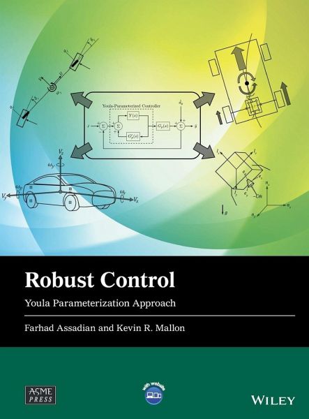
Robust Control Robust Control Youla Parameterization Approach Discover efficient methods for designing robust control systems In Robust Control: Youla Parameterization Approach, accomplished engineers Dr. Farhad Assadian and Kevin R. Mallon deliver an insightful treatment of robust control system design that does not require a theoretical background in controls. The authors connect classical control theory to modern control concepts using the Youla method and offer practical examples from the automotive industry for designing control systems with the Youla method. The book demonstrates that…mehr
Andere Kunden interessierten sich auch für
- Philippe FeyelRobust Control Optimization with Metaheuristics186,99 €
- Jürgen AckermannRobust Control271,99 €
- Yugeng XiPredictive Control156,99 €
- Mark Graves / Bruce Batchelor (eds.)Machine Vision for the Inspection of Natural Products184,99 €
- Isabelle FantoniNon-Linear Control for Underactuated Mechanical Systems109,99 €
- Wodek K. GawronskiAdvanced Structural Dynamics and Active Control of Structures278,99 €
- Jan M. SkowronskiControl of Nonlinear Mechanical Systems143,99 €
-
-
-
Robust Control Robust Control Youla Parameterization Approach Discover efficient methods for designing robust control systems In Robust Control: Youla Parameterization Approach, accomplished engineers Dr. Farhad Assadian and Kevin R. Mallon deliver an insightful treatment of robust control system design that does not require a theoretical background in controls. The authors connect classical control theory to modern control concepts using the Youla method and offer practical examples from the automotive industry for designing control systems with the Youla method. The book demonstrates that feedback control can be elegantly designed in the frequency domain using the Youla parameterization approach. It offers deep insights into the many practical applications from utilizing this technique in both Single Input Single Output (SISO) and Multiple Input Multiple Output (MIMO) design. Finally, the book provides an estimation technique using Youla parameterization and controller output observer for the first time. Robust Control offers readers: * A thorough introduction to a review of the Laplace Transform, including singularity functions and transfer functions * Comprehensive explorations of the response of linear, time-invariant, and dynamic systems, as well as feedback principles and feedback design for SISO * Practical discussions of norms and feedback systems, feedback design by the optimization of closed-loop norms, and estimation design for SISO using the parameterization approach * In-depth examinations of MIMO control and multivariable transfer function properties Perfect for industrial researchers and engineers working with control systems, Robust Control: Youla Parameterization Approach is also an indispensable resource for graduate students in mechanical, aerospace, electrical, and chemical engineering.
Hinweis: Dieser Artikel kann nur an eine deutsche Lieferadresse ausgeliefert werden.
Produktdetails
- Produktdetails
- Verlag: Wiley
- Seitenzahl: 464
- Erscheinungstermin: 7. Februar 2022
- Englisch
- Abmessung: 286mm x 221mm x 29mm
- Gewicht: 1415g
- ISBN-13: 9781119500360
- ISBN-10: 1119500362
- Artikelnr.: 62435090
- Verlag: Wiley
- Seitenzahl: 464
- Erscheinungstermin: 7. Februar 2022
- Englisch
- Abmessung: 286mm x 221mm x 29mm
- Gewicht: 1415g
- ISBN-13: 9781119500360
- ISBN-10: 1119500362
- Artikelnr.: 62435090
Farhad Assadian, PhD, is Professor of Dynamic Systems and Control in the Department of Mechanical and Aerospace Engineering at the University of California, Davis. He teaches courses on dynamics, modelling and simulation, and control theory. Kevin R. Mallon is a PhD student in the Department of Mechanical and Aerospace Engineering at the University of California, Davis. He previously worked as a robotics engineer at Intelligrated Systems.
Preface xv Acknowledgments xix Introduction xxi About the Companion Website xxix Part I Control Design Using Youla Parameterization: Single Input Single Output (SISO) 1 1 Review of the Laplace Transform 3 1.1 The Laplace Transform Concept 3 1.2 Singularity Functions 3 1.2.1 Definition of the Impulse Function 4 1.2.2 The Impulse Function and the Riemann Integral 5 1.2.3 The General Definition of Singularity Functions 5 1.2.3.1 "Graphs" of Some Singularity Functions 5 1.3 The Laplace Transform 7 1.3.1 Definition of the Laplace Transform 7 1.3.2 Laplace Transform Properties 8 1.3.3 Shifting the Laplace Transform 8 1.3.4 Laplace Transform Derivatives 10 1.3.5 Transforms of Singularity Functions 12 1.4 Inverse Laplace Transform 13 1.4.1 Inverse Laplace Transformation by Heaviside Expansion 13 1.4.1.1 Distinct Poles 13 1.4.1.2 Distinct Poles with G(s) Being Proper 13 1.4.1.3 Repeated Poles 14 1.5 The Transfer Function and the State Space Representations (State Equations) 16 1.5.1 The Transfer Function 16 1.5.2 The State Equations 16 1.5.3 Transfer Function Properties 17 1.5.4 Poles and Zeros of a Transfer Function 18 1.5.5 Physical Realizability 19 1.6 Problems 21 2 The Response of Linear, Time-Invariant Dynamic Systems 25 2.1 The Time Response of Dynamic Systems 25 2.1.1 Final Value Theorem 25 2.1.2 Initial Value Theorem 26 2.1.3 Convolution and the Laplace Transform 27 2.1.4 Transmission Blocking Response 29 2.1.5 Stability 31 2.1.6 Initial Values and Reverse Action 35 2.1.7 Final Values and Static Gain 36 2.1.8 Time Response Metrics 38 2.1.8.1 First-Order System (Single-Pole Response) 38 2.1.8.2 Second-Order System (Quadratic Factor) 39 2.1.9 The Effect of Zeros on Transient Response 41 2.1.10 The Butterworth Pattern 42 2.2 Frequency Response of Dynamic Systems 43 2.2.1 Steady-State Frequency Response of LTI systems 43 2.2.2 Frequency Response Representation 45 2.2.3 Frequency Response: The Real Pole 45 2.2.4 Frequency Response: The Real Zero 47 2.2.5 Frequency Response: The Quadratic Factor 49 2.2.6 Frequency Response: Pure Time Delay 50 2.2.7 Frequency Response: Static Gain 53 2.2.8 Frequency Response: The Composite Transfer Function 53 2.2.9 Frequency Response: Asymptote Formulas 54 2.2.10 Physical Realizability 54 2.2.11 Non-minimum Phase, All-Pass, and Blaschke Factors 55 2.3 Frequency Response Plotting 55 2.3.1 Matlab Codes for Plotting System Frequency Response 56 2.3.1.1 Bode Plot 56 2.3.1.2 Polar Plot/Nyquist Diagram 56 2.4 Problems 57 3 Feedback Principals 61 3.1 The Value of Feedback Control 62 3.1.1 The Advantages of the Closed Loop 63 3.2 Closed-Loop Transfer Functions 64 3.2.1 The Return Ratio 65 3.2.2 Closed-Loop Transfer Functions and the Return Difference 65 3.2.3 Sensitivity, Complementary Sensitivity, and the Youla Parameter 66 3.3 Well-Posedness and Internal Stability 70 3.3.1 Well-Posedness 70 3.3.2 The Internal Stability of Feedback Control 71 3.3.2.1 The Closed-Loop Characteristic Equation and Closed-Loop Poles 72 3.3.2.2 Closed-Loop Zeros 72 3.3.2.3 Pole-Zero Cancellation and The Internal Stability of Feedback Control 73 3.4 The Youla Parameterization of all Internally Stabilizing Compensators 76 3.5 Interpolation Conditions 80 3.6 Steady-State Error 83 3.7 Feedback Design, and Frequency Methods: Input Attenuation and Robustness 83 3.7.1 The Frequency Paradigm 84 3.7.2 Input Attenuation and Command Following 84 3.7.3 Bode Measures of Performance Robustness 85 3.7.4 Graphical Interpretation of Return, Sensitivity, and Complementary Sensitivity 88 3.7.5 Weighting Factors and Performance Robustness 89 3.8 The Saturation Constraints 90 3.8.1 Bandwidth and Response Time 90 3.8.2 The Youla Parameter and Saturation 91 3.9 Problems 93 4 Feedback Design For SISO: Shaping and Parameterization 95 4.1 Closed-Loop Stability Under Uncertain Conditions 95 4.1.1 Harmonic Consistency 95 4.1.2 Nyquist Stability Criterion: Heuristic Justification 96 4.1.3 Stability Margins and Stability Robustness 98 4.1.4 Margins, T(j
) and S(j
), and H
Norms (Relationships Between Classical and Neoclassical Approaches) 99 4.1.4.1 Neoclassical Approach 101 4.2 Mathematical Design Constraints 103 4.2.1 Sensitivity/Complementary Sensitivity Point-wise Constraints 103 4.2.2 Sensitivity, Complementary Sensitivity, and Analytic Constraints 104 4.2.2.1 Non-minimum Phase Constraints on Design 104 4.3 The Neoclassical Approach to Internal Stability 104 4.4 Feedback Design And Parameterization: Stable Objects 106 4.4.1 Renormalization of Gains 108 4.4.2 Shaping of the Closed-Loop: Stable SISO 108 4.4.3 Neoclassical Design Principles 109 4.5 Loop Shaping Using Youla Parameterization 110 4.5.1 LHP Zeros of Gp 111 4.5.2 Non-minimum Phase Zeros 112 4.5.3 LHP Poles of Gp 114 4.5.4 Unstable Poles 115 4.6 Design Guidelines 116 4.7 Design Examples 117 4.8 Problems 125 5 Norms of Feedback Systems 129 5.1 The Laplace and Fourier Transform 129 5.1.1 The Inverse Laplace Transform 129 5.1.2 Parseval's Theorem 131 5.1.3 The Fourier Transform 132 5.1.3.1 Properties of the Fourier Transform 133 5.1.3.2 Inverse Fourier Transformation By Heaviside Expansion 133 5.2 Norms of Signals and Systems 134 5.2.1 Signal Norms 134 5.2.1.1 Particular Norms 135 5.2.1.2 Properties of Norms 136 5.2.2 Norms of Dynamic Systems 137 5.2.3 Input-Output Norms 138 5.2.3.1 Transient Inputs (Energy Bounded) 138 5.2.3.2 Persistent Inputs (Energy Unbounded) 139 5.3 Quantifying Uncertainty 140 5.3.1 The Characterization of Uncertainty in Models 140 5.3.2 Weighting Factors and Stability Robustness 141 5.3.3 Robust Stability (Complementary Sensitivity) and Uncertainty 142 5.3.4 Sensitivity and Performance 145 5.3.5 Performance and Stability 146 5.4 Problems 147 6 Feedback Design By the Optimization of Closed-Loop Norms 149 6.1 Introduction 149 6.1.1 Frequency Domain Control Design Approaches 150 6.2 Optimization Design Objectives and Constraints 151 6.2.1 Algebraic Constraints 151 6.2.2 Analytic Constraints 152 6.2.2.1 Nonminimum Phase Effect 152 6.2.2.2 Bode Sensitivity Integral Theorem 153 6.3 The Linear Fractional Transformation 154 6.4 Setup for Loop-Shaping Optimization 156 6.4.1 Setup for Youla Parameter Loop Shaping 158 6.5 H
-norm Optimization Problem 160 6.5.1 Solution to a Simple Optimization Problem 161 6.6 H
Design 163 6.7 H
Solutions Using Matlab Robust Control Toolbox for SISO Systems 164 6.7.1 Defining Frequency Weights 164 6.8 Problems 168 7 Estimation Design for SISO Using Parameterization Approach 173 7.1 Introduction 173 7.2 Youla Controller Output Observer Concept 175 7.3 The SISO Case 177 7.3.1 Output and Feedthrough Matrices 178 7.3.2 SISO Estimator Design 178 7.4 Final Remarks 182 8 Practical Applications 183 8.1 Yaw Stability Control with Active Limited Slip Differential 183 8.1.1 Model and Control Design 183 8.1.2 Youla Control Design Using Hand Computation 187 8.1.3 H
Control Design Using Loop-shaping Technique 188 8.2 Vehicle Yaw Rate and Side-Slip Estimation 195 8.2.1 Kalman Filters 195 8.2.2 Vehicle Model - Nonlinear Bicycle Model with Pacejka Tire Model 196 8.2.3 Linearizing the Bicycle Model 197 8.2.4 Uncertainties 197 8.2.5 State Estimation 198 8.2.6 Youla Parameterization Estimator Design 198 8.2.7 Simulation Results 200 8.2.8 Robustness Test 201 8.2.8.1 Vehicle Mass Variation 201 8.2.8.2 Tire-road Coefficient of Friction 203 Part II Control Design Using Youla Parametrization: Multi Input Multi Output (MIMO) 205 9 Introduction to Multivariable Feedback Control 207 9.1 Nonoptimal, Optimal, and Robust Control 207 9.1.1 Nonoptimal Control Methods 208 9.1.2 Optimal Control Methods 208 9.1.3 Optimal Robust Control 209 9.2 Review of the SISO Transfer Function 210 9.2.1 Schur Complement 210 9.2.2 Interpretation of Poles and Zeros of a Transfer Function 211 9.2.2.1 Poles 211 9.2.2.2 Zeros 212 9.2.2.3 Transmission Blocking Zeros 213 9.3 Basic Aspects of Transfer Function Matrices 215 9.4 Problems 215 10 Matrix Fractional Description 217 10.1 Transfer Function Matrices 217 10.1.1 Matrix Fraction Description 218 10.2 Polynomial Matrix Properties 219 10.2.1 Minimum-Degree Factorization 220 10.3 Equivalency of Polynomial Matrices 221 10.4 Smith Canonical Form 222 10.5 Smith-McMillan Form 225 10.5.1 Smith-McMillan Form 225 10.5.2 MFD's and Their Relations to Smith-McMillan Form 228 10.5.3 Computing an Irreducible (Coprime) Matrix Fraction Description 229 10.6 MIMO Controllability and Observability 234 10.6.1 State-Space Realization 235 10.6.1.1 SISO System 235 10.6.1.2 MIMO System 236 10.6.2 Controllable Form of State-Space Realization of MIMO System 238 10.6.2.1 Mathematical Details 239 10.7 Straightforward Computational Procedures 243 10.8 Problems 245 11 Eigenvalues and Singular Values 247 11.1 Eigenvalues and Eigenvectors 247 11.2 Matrix Diagonalization 248 11.2.1 Classes of Diagonalizable Matrices 250 11.3 Singular Value Decomposition 253 11.3.1 What is a Singular Value Decomposition? 254 11.3.2 Orthonormal Vectors 255 11.4 Singular Value Decomposition Properties 257 11.5 Comparison of Eigenvalue and Singular Value Decompositions 258 11.5.1 System Gain 259 11.6 Generalized Singular Value Decomposition 262 11.6.1 The Scalar Case 264 11.6.2 Input and Output Spaces 264 11.7 Norms 265 11.7.1 The Spectral Norm 265 11.8 Problems 266 12 MIMO Feedback Principals 267 12.1 Mutlivariable Closed-Loop Transfer Functions 267 12.1.1 Transfer Function Matrix, From r to y 268 12.1.2 Transfer Function Matrix From dy to y As Shown in Figure 12.1 268 12.1.3 Transfer Function Matrix From r to e 269 12.1.4 Transfer Function From r to u 269 12.1.5 Realization Tricks 270 12.2 Well-Posedness of MIMO Systems 270 12.3 State Variable Compositions 271 12.4 Nyquist Criterion for MIMO Systems 273 12.4.1 Characteristic Gains 273 12.4.2 Poles and Zeros 274 12.4.3 Internal Stability 275 12.5 MIMO Performance and Robustness Criteria 276 12.6 Open-Loop Singular Values 278 12.6.1 Crossover Frequency 279 12.6.2 Bandwidth Constraints 280 12.7 Condition Number and its Role in MIMO Control Design 281 12.7.1 Condition Numbers and Decoupling 281 12.7.2 Role of Tu and S u in MIMO Feedback Design 282 12.8 Summary of Requirements 282 12.8.1 Closed-Loop Requirements 282 12.8.2 Open-Loop Requirements 283 12.9 Problems 283 13 Youla Parameterization for Feedback Systems 285 13.1 Neoclassical Control for MIMO Systems 285 13.1.1 Internal Model Control 285 13.2 MIMO Feedback Control Design for Stable Plants 286 13.2.1 Procedure to Find the MIMO Controller, G c 287 13.2.2 Interpolation Conditions 287 13.3 MIMO Feedback Control Design Examples 287 13.3.1 Summary of Closed-Loop Requirements 290 13.3.2 Summary of Open-Loop Requirements 290 13.4 MIMO Feedback Control Design: Unstable Plants 294 13.4.1 The Proposed Control Design Method 294 13.4.2 Another Approach for MIMO Controller Design 300 13.5 Problems 301 14 Norms of Feedback Systems 303 14.1 Norms 303 14.1.1 Signal Norms, the Discrete Case 303 14.1.2 System Norms 304 14.1.3 The
2-Norm 305 14.1.4 The
-Norm 306 14.2 Linear Fractional Transformations (LFT) 307 14.3 Linear Fractional Transformation Explained 309 14.3.1 LFTs in Control Design 310 14.4 Modeling Uncertainties 312 14.4.1 Uncertainties 312 14.4.2 Descriptions of Unstructured Uncertainty 312 14.5 General Robust Stability Theorem 313 14.5.1 SVD Properties Applied 314 14.5.2 Robust Performance 315 14.6 Problems 316 15 Optimal Control in MIMO Systems 319 15.1 Output Feedback Control 319 15.1.1 LQG Control 320 15.1.2 Kalman Filter 322 15.1.3
2 Control 323 15.1.3.1 Kalman Filter Dynamic Model 324 15.1.3.2 State Feedback 325 15.2
Control Design 325 15.2.1 State Feedback (Full Information)
Control Design 327 15.2.2
Filtering 329 15.3
- Robust Optimal Control 330 15.4 Problems 332 16 Estimation Design for MIMO Using Parameterization Approach 335 16.1 YCOO Concept for MIMO 335 16.2 MIMO Estimator Design 337 16.3 State Estimation 338 16.3.1 First Decoupled System ( Gsm 1 ) 338 16.3.2 Second Decoupled System ( Gsm 2 ) 338 16.3.3 Coupled System 339 16.4 Applications 339 16.4.1 States Estimation: Four States 340 16.4.2 Input Estimation: Skyhook Based Control 341 16.4.3 Input Estimation: Road Roughness 342 16.5 Final Remarks 344 17 Practical Applications 345 17.1 Active Suspension 345 17.1.1 Model and Control Design 345 17.1.2 MIMO Youla Control Design 348 17.1.3 H
Control Design Technique 350 17.1.4 Uncertain Actuator Model 351 17.1.5 Design Setup 351 17.1.6 Simulation Results 354 17.1.7 Robustness Test: Actuator Model Variations 356 17.2 Advanced Engine Speed Control for Hybrid Vehicles 356 17.2.1 Diesel Hybrid Electric Vehicle Model 357 17.2.2 MISO Youla Control Design 359 17.2.3 First Youla Method 359 17.2.4 Second Youla Method 360 17.2.5 H
Control Design 360 17.2.6 Simulation Results 362 17.2.7 Robustness Test 363 17.3 Robust Control for the Powered Descent of a Multibody Lunar Landing System 364 17.3.1 Multibody Dynamics Model 365 17.3.2 Trajectory Optimization 366 17.3.3 MIMO Youla Control Design 367 17.3.4 Youla Method for Under-Actuated Systems 371 17.4 Vehicle Yaw Rate and Sideslip Estimation 374 17.4.1 Background 375 17.4.2 Vehicle Modeling 376 17.4.2.1 Nonlinear Bicycle Model With Pacejka Tire Model 376 17.4.2.2 Kinematic Relationship 376 17.4.2.3 Multi-Input Model 377 17.4.2.4 Linearizing the Bicycle Model for SISO and MIMO Cases 378 17.4.3 State Estimation 378 17.4.3.1 Youla Parameterization Control Design 378 17.4.4 Simulation and Estimation Result 379 17.4.5 Robustness Test 382 17.4.5.1 Vehicle mass variation 382 17.4.5.2 Tire-road coefficient of friction 382 17.4.6 Sensor Bias 382 17.4.7 Final Remarks 386 A Cauchy Integral 387 A.1 Contour Definitions 387 A.2 Contour Integrals 388 A.3 Complex Analysis Definitions 389 A.4 Cauchy-Riemann Conditions 390 A.5 Cauchy Integral Theorem 392 A.5.1 Terminology 394 A.6 Maximum Modulus Theorem 394 A.7 Poisson Integral Formula 396 A.8 Cauchy's Argument Principle 398 A.9 Nyquist Stability Criterion 400 B Singular Value Properties 403 B.1 Spectral Norm Proof 403 B.2 Proof of Bounded Eigenvalues 404 B.3 Proof of Matrix Inequality 404 B.3.1 Upper Bound 405 B.3.2 Lower Bound 405 B.3.3 Combined Inequality 406 B.4 Triangle Inequality 406 B.4.1 Upper Bound 406 B.4.2 Lower Bound 406 B.4.3 Combined Inequality 406 C Bandwidth 407 C.1 Introduction 407 C.2 Information as a Precise Measure of Bandwidth 408 C.2.1 Neoclassical Feedback Control 408 C.2.2 Defining a Measure to Characterize the Usefulness of Feedback 408 C.2.3 Computation of New Bandwidth 409 C.3 Examples 410 C.4 Summary 414 D Example Matlab Code 417 D.1 Example 1 417 D.2 Example 2 419 D.3 Example 3 420 D.4 Example 4 422 References 425 Index 427