Peter M. Lee

Bayesian Statistics (eBook, PDF)

An Introduction

• Format: PDF

Produktbeschreibung

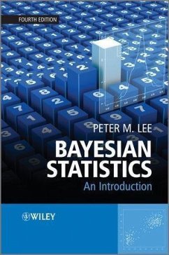
Bayesian Statistics is the school of thought that combines prior beliefs with the likelihood of a hypothesis to arrive at posterior beliefs. The first edition of Peter Lee's book appeared in 1989, but the subject has moved ever onwards, with increasing emphasis on Monte Carlo based techniques. This new fourth edition looks at recent techniques such as variational methods, Bayesian importance sampling, approximate Bayesian computation and Reversible Jump Markov Chain Monte Carlo (RJMCMC), providing a concise account of the way in which the Bayesian approach to statistics develops as well as how it contrasts with the conventional approach. The theory is built up step by step, and important notions such as sufficiency are brought out of a discussion of the salient features of specific examples. This edition: * Includes expanded coverage of Gibbs sampling, including more numerical examples and treatments of OpenBUGS, R2WinBUGS and R2OpenBUGS. * Presents significant new material on recent techniques such as Bayesian importance sampling, variational Bayes, Approximate Bayesian Computation (ABC) and Reversible Jump Markov Chain Monte Carlo (RJMCMC). * Provides extensive examples throughout the book to complement the theory presented. * Accompanied by a supporting website featuring new material and solutions. More and more students are realizing that they need to learn Bayesian statistics to meet their academic and professional goals. This book is best suited for use as a main text in courses on Bayesian statistics for third and fourth year undergraduates and postgraduate students.

---

Dieser Download kann aus rechtlichen Gründen nur mit Rechnungsadresse in A, B, BG, CY, CZ, D, DK, EW, E, FIN, F, GR, HR, H, IRL, I, LT, L, LR, M, NL, PL, P, R, S, SLO, SK ausgeliefert werden.

Produktdetails

• Verlag: John Wiley & Sons
• Seitenzahl: 488
• Erscheinungstermin: 12. Juni 2012
• Englisch
• ISBN-13: 9781118359754
• Artikelnr.: 37354138

Autorenporträt

Peter Lee, Department of Mathematics & Formerly Provost of Wentworth College, University of York.

Inhaltsangabe

Preface xix
Preface to the First Edition xxi
1 Preliminaries 1
1.1 Probability and Bayes' Theorem 1
1.1.1 Notation 1
1.1.2 Axioms for probability 2
1.1.3 'Unconditional' probability 5
1.1.4 Odds 6
1.1.5 Independence 7
1.1.6 Some simple consequences of the axioms; Bayes' Theorem 7
1.2 Examples on Bayes' Theorem 9
1.2.1 The Biology of Twins 9
1.2.2 A political example 10
1.2.3 A warning 10
1.3 Random variables 12
1.3.1 Discrete random variables 12
1.3.2 The binomial distribution 13
1.3.3 Continuous random variables 14
1.3.4 The normal distribution 16
1.3.5 Mixed random variables 17
1.4 Several random variables 17
1.4.1 Two discrete random variables 17
1.4.2 Two continuous random variables 18
1.4.3 Bayes' Theorem for random variables 20
1.4.4 Example 21
1.4.5 One discrete variable and one continuous variable 21
1.4.6 Independent random variables 22
1.5 Means and variances 23
1.5.1 Expectations 23
1.5.2 The expectation of a sum and of a product 24
1.5.3 Variance, precision and standard deviation 25
1.5.4 Examples 25
1.5.5 Variance of a sum; covariance and correlation 27
1.5.6 Approximations to the mean and variance of a function of a random
variable 28
1.5.7 Conditional expectations and variances 29
1.5.8 Medians and modes 31
1.6 Exercises on Chapter 1 31
2 Bayesian inference for the normal distribution 36
2.1 Nature of Bayesian inference 36
2.1.1 Preliminary remarks 36
2.1.2 Post is prior times likelihood 36
2.1.3 Likelihood can be multiplied by any constant 38
2.1.4 Sequential use of Bayes' Theorem 38
2.1.5 The predictive distribution 39
2.1.6 A warning 39
2.2 Normal prior and likelihood 40
2.2.1 Posterior from a normal prior and likelihood 40
2.2.2 Example 42
2.2.3 Predictive distribution 43
2.2.4 The nature of the assumptions made 44
2.3 Several normal observations with a normal prior 44
2.3.1 Posterior distribution 44
2.3.2 Example 46
2.3.3 Predictive distribution 47
2.3.4 Robustness 47
2.4 Dominant likelihoods 48
2.4.1 Improper priors 48
2.4.2 Approximation of proper priors by improper priors 49
2.5 Locally uniform priors 50
2.5.1 Bayes' postulate 50
2.5.2 Data translated likelihoods 52
2.5.3 Transformation of unknown parameters 52
2.6 Highest density regions 54
2.6.1 Need for summaries of posterior information 54
2.6.2 Relation to classical statistics 55
2.7 Normal variance 55
2.7.1 A suitable prior for the normal variance 55
2.7.2 Reference prior for the normal variance 58
2.8 HDRs for the normal variance 59
2.8.1 What distribution should we be considering? 59
2.8.2 Example 59
2.9 The role of sufficiency 60
2.9.1 Definition of sufficiency 60
2.9.2 Neyman's factorization theorem 61
2.9.3 Sufficiency principle 63
2.9.4 Examples 63
2.9.5 Order statistics and minimal sufficient statistics 65
2.9.6 Examples on minimal sufficiency 66
2.10 Conjugate prior distributions 67
2.10.1 Definition and difficulties 67
2.10.2 Examples 68
2.10.3 Mixtures of conjugate densities 69
2.10.4 Is your prior really conjugate? 71
2.11 The exponential family 71
2.11.1 Definition 71
2.11.2 Examples 72
2.11.3 Conjugate densities 72
2.11.4 Two-parameter exponential family 73
2.12 Normal mean and variance both unknown 73
2.12.1 Formulation of the problem 73
2.12.2 Marginal distribution of the mean 75
2.12.3 Example of the posterior density for the mean 76
2.12.4 Marginal distribution of the variance 77
2.12.5 Example of the posterior density of the variance 77
2.12.6 Conditional density of the mean for given variance 77
2.13 Conjugate joint prior for the normal distribution 78
2.13.1 The form of the conjugate prior 78
2.13.2 Derivation of the posterior 80
2.13.3 Example 81
2.13.4 Concluding remarks 82
2.14 Exercises on Chapter 2 82
3 Some other common distributions 85
3.1 The binomial distribution 85
3.1.1 Conjugate prior 85
3.1.2 Odds and log-odds 88
3.1.3 Highest density regions 90
3.1.4 Example 91
3.1.5 Predictive distribution 92
3.2 Reference prior for the binomial likelihood 92
3.2.1 Bayes' postulate 92
3.2.2 Haldane's prior 93
3.2.3 The arc-sine distribution 94
3.2.4 Conclusion 95
3.3 Jeffreys' rule 96
3.3.1 Fisher's information 96
3.3.2 The information from several observations 97
3.3.3 Jeffreys' prior 98
3.3.4 Examples 98
3.3.5 Warning 100
3.3.6 Several unknown parameters 100
3.3.7 Example 101
3.4 The Poisson distribution 102
3.4.1 Conjugate prior 102
3.4.2 Reference prior 103
3.4.3 Example 104
3.4.4 Predictive distribution 104
3.5 The uniform distribution 106
3.5.1 Preliminary definitions 106
3.5.2 Uniform distribution with a fixed lower endpoint 107
3.5.3 The general uniform distribution 108
3.5.4 Examples 110
3.6 Reference prior for the uniform distribution 110
3.6.1 Lower limit of the interval fixed 110
3.6.2 Example 111
3.6.3 Both limits unknown 111
3.7 The tramcar problem 113
3.7.1 The discrete uniform distribution 113
3.8 The first digit problem; invariant priors 114
3.8.1 A prior in search of an explanation 114
3.8.2 The problem 114
3.8.3 A solution 115
3.8.4 Haar priors 117
3.9 The circular normal distribution 117
3.9.1 Distributions on the circle 117
3.9.2 Example 119
3.9.3 Construction of an HDR by numerical integration 120
3.9.4 Remarks 122
3.10 Approximations based on the likelihood 122
3.10.1 Maximum likelihood 122
3.10.2 Iterative methods 123
3.10.3 Approximation to the posterior density 123
3.10.4 Examples 124
3.10.5 Extension to more than one parameter 126
3.10.6 Example 127
3.11 Reference posterior distributions 128
3.11.1 The information provided by an experiment 128
3.11.2 Reference priors under asymptotic normality 130
3.11.3 Uniform distribution of unit length 131
3.11.4 Normal mean and variance 132
3.11.5 Technical complications 134
3.12 Exercises on Chapter 3 134
4 Hypothesis testing 138
4.1 Hypothesis testing 138
4.1.1 Introduction 138
4.1.2 Classical hypothesis testing 138
4.1.3 Difficulties with the classical approach 139
4.1.4 The Bayesian approach 140
4.1.5 Example 142
4.1.6 Comment 143
4.2 One-sided hypothesis tests 143
4.2.1 Definition 143
4.2.2 P-values 144
4.3 Lindley's method 145
4.3.1 A compromise with classical statistics 145
4.3.2 Example 145
4.3.3 Discussion 146
4.4 Point (or sharp) null hypotheses with prior information 146
4.4.1 When are point null hypotheses reasonable? 146
4.4.2 A case of nearly constant likelihood 147
4.4.3 The Bayesian method for point null hypotheses 148
4.4.4 Sufficient statistics 149
4.5 Point null hypotheses for the normal distribution 150
4.5.1 Calculation of the Bayes' factor 150
4.5.2 Numerical examples 151
4.5.3 Lindley's paradox 152
4.5.4 A bound which does not depend on the prior distribution 154
4.5.5 The case of an unknown variance 155
4.6 The Doogian philosophy 157
4.6.1 Description of the method 157
4.6.2 Numerical example 157
4.7 Exercises on Chapter 4 158
5 Two-sample problems 162
5.1 Two-sample problems - both variances unknown 162
5.1.1 The problem of two normal samples 162
5.1.2 Paired comparisons 162
5.1.3 Example of a paired comparison problem 163
5.1.4 The case where both variances are known 163
5.1.5 Example 164
5.1.6 Non-trivial prior information 165
5.2 Variances unknown but equal 165
5.2.1 Solution using reference priors 165
5.2.2 Example 167
5.2.3 Non-trivial prior information 167
5.3 Variances unknown and unequal (Behrens-Fisher problem) 168
5.3.1 Formulation of the problem 168
5.3.2 Patil's approximation 169
5.3.3 Example 170
5.3.4 Substantial prior information 170
5.4 The Behrens-Fisher controversy 171
5.4.1 The Behrens-Fisher problem from a classical standpoint 171
5.4.2 Example 172
5.4.3 The controversy 173
5.5 Inferences concerning a variance ratio 173
5.5.1 Statement of the problem 173
5.5.2 Derivation of the F distribution 174
5.5.3 Example 175
5.6 Comparison of two proportions; the 2 × 2 table 176
5.6.1 Methods based on the log-odds ratio 176
5.6.2 Example 177
5.6.3 The inverse root-sine transformation 178
5.6.4 Other methods 178
5.7 Exercises on Chapter 5 179
6 Correlation, regression and the analysis of variance 182
6.1 Theory of the correlation coefficient 182
6.1.1 Definitions 182
6.1.2 Approximate posterior distribution of the correlation coefficient 184
6.1.3 The hyperbolic tangent substitution 186
6.1.4 Reference prior 188
6.1.5 Incorporation of prior information 189
6.2 Examples on the use of the correlation coefficient 189
6.2.1 Use of the hyperbolic tangent transformation 189
6.2.2 Combination of several correlation coefficients 189
6.2.3 The squared correlation coefficient 190
6.3 Regression and the bivariate normal model 190
6.3.1 The model 190
6.3.2 Bivariate linear regression 191
6.3.3 Example 193
6.3.4 Case of known variance 194
6.3.5 The mean value at a given value of the explanatory variable 194
6.3.6 Prediction of observations at a given value of the explanatory
variable 195
6.3.7 Continuation of the example 195
6.3.8 Multiple regression 196
6.3.9 Polynomial regression 196
6.4 Conjugate prior for the bivariate regression model 197
6.4.1 The problem of updating a regression line 197
6.4.2 Formulae for recursive construction of a regression line 197
6.4.3 Finding an appropriate prior 199
6.5 Comparison of several means - the one way model 200
6.5.1 Description of the one way layout 200
6.5.2 Integration over the nuisance parameters 201
6.5.3 Derivation of the F distribution 203
6.5.4 Relationship to the analysis of variance 203
6.5.5 Example 204
6.5.6 Relationship to a simple linear regression model 206
6.5.7 Investigation of contrasts 207
6.6 The two way layout 209
6.6.1 Notation 209
6.6.2 Marginal posterior distributions 210
6.6.3 Analysis of variance 212
6.7 The general linear model 212
6.7.1 Formulation of the general linear model 212
6.7.2 Derivation of the posterior 214
6.7.3 Inference for a subset of the parameters 215
6.7.4 Application to bivariate linear regression 216
6.8 Exercises on Chapter 6 217
7 Other topics 221
7.1 The likelihood principle 221
7.1.1 Introduction 221
7.1.2 The conditionality principle 222
7.1.3 The sufficiency principle 223
7.1.4 The likelihood principle 223
7.1.5 Discussion 225
7.2 The stopping rule principle 226
7.2.1 Definitions 226
7.2.2 Examples 226
7.2.3 The stopping rule principle 227
7.2.4 Discussion 228
7.3 Informative stopping rules 229
7.3.1 An example on capture and recapture of fish 229
7.3.2 Choice of prior and derivation of posterior 230
7.3.3 The maximum likelihood estimator 231
7.3.4 Numerical example 231
7.4 The likelihood principle and reference priors 232
7.4.1 The case of Bernoulli trials and its general implications 232
7.4.2 Conclusion 233
7.5 Bayesian decision theory 234
7.5.1 The elements of game theory 234
7.5.2 Point estimators resulting from quadratic loss 236
7.5.3 Particular cases of quadratic loss 237
7.5.4 Weighted quadratic loss 238
7.5.5 Absolute error loss 238
7.5.6 Zero-one loss 239
7.5.7 General discussion of point estimation 240
7.6 Bayes linear methods 240
7.6.1 Methodology 240
7.6.2 Some simple examples 241
7.6.3 Extensions 243
7.7 Decision theory and hypothesis testing 243
7.7.1 Relationship between decision theory and classical hypothesis testing
243
7.7.2 Composite hypotheses 245
7.8 Empirical Bayes methods 245
7.8.1 Von Mises' example 245
7.8.2 The Poisson case 246
7.9 Exercises on Chapter 7 247
8 Hierarchical models 253
8.1 The idea of a hierarchical model 253
8.1.1 Definition 253
8.1.2 Examples 254
8.1.3 Objectives of a hierarchical analysis 257
8.1.4 More on empirical Bayes methods 257
8.2 The hierarchical normal model 258
8.2.1 The model 258
8.2.2 The Bayesian analysis for known overall mean 259
8.2.3 The empirical Bayes approach 261
8.3 The baseball example 262
8.4 The Stein estimator 264
8.4.1 Evaluation of the risk of the James-Stein estimator 267
8.5 Bayesian analysis for an unknown overall mean 268
8.5.1 Derivation of the posterior 270
8.6 The general linear model revisited 272
8.6.1 An informative prior for the general linear model 272
8.6.2 Ridge regression 274
8.6.3 A further stage to the general linear model 275
8.6.4 The one way model 276
8.6.5 Posterior variances of the estimators 277
8.7 Exercises on Chapter 8 277
9 The Gibbs sampler and other numerical methods 281
9.1 Introduction to numerical methods 281
9.1.1 Monte Carlo methods 281
9.1.2 Markov chains 282
9.2 The EM algorithm 283
9.2.1 The idea of the EM algorithm 283
9.2.2 Why the EM algorithm works 285
9.2.3 Semi-conjugate prior with a normal likelihood 287
9.2.4 The EM algorithm for the hierarchical normal model 288
9.2.5 A particular case of the hierarchical normal model 290
9.3 Data augmentation by Monte Carlo 291
9.3.1 The genetic linkage example revisited 291
9.3.2 Use of R 291
9.3.3 The genetic linkage example in R 292
9.3.4 Other possible uses for data augmentation 293
9.4 The Gibbs sampler 294
9.4.1 Chained data augmentation 294
9.4.2 An example with observed data 296
9.4.3 More on the semi-conjugate prior with a normal likelihood 299
9.4.4 The Gibbs sampler as an extension of chained data augmentation 301
9.4.5 An application to change-point analysis 302
9.4.6 Other uses of the Gibbs sampler 306
9.4.7 More about convergence 309
9.5 Rejection sampling 311
9.5.1 Description 311
9.5.2 Example 311
9.5.3 Rejection sampling for log-concave distributions 311
9.5.4 A practical example 313
9.6 The Metropolis-Hastings algorithm 317
9.6.1 Finding an invariant distribution 317
9.6.2 The Metropolis-Hastings algorithm 318
9.6.3 Choice of a candidate density 320
9.6.4 Example 321
9.6.5 More realistic examples 322
9.6.6 Gibbs as a special case of Metropolis-Hastings 322
9.6.7 Metropolis within Gibbs 323
9.7 Introduction to WinBUGS and OpenBUGS 323
9.7.1 Information about WinBUGS and OpenBUGS 323
9.7.2 Distributions in WinBUGS and OpenBUGS 324
9.7.3 A simple example using WinBUGS 324
9.7.4 The pump failure example revisited 327
9.7.5 DoodleBUGS 327
9.7.6 coda 329
9.7.7 R2WinBUGS and R2OpenBUGS 329
9.8 Generalized linear models 332
9.8.1 Logistic regression 332
9.8.2 A general framework 334
9.9 Exercises on Chapter 9 335
10 Some approximate methods 340
10.1 Bayesian importance sampling 340
10.1.1 Importance sampling to find HDRs 343
10.1.2 Sampling importance re-sampling 344
10.1.3 Multidimensional applications 344
10.2 Variational Bayesian methods: simple case 345
10.2.1 Independent parameters 347
10.2.2 Application to the normal distribution 349
10.2.3 Updating the mean 350
10.2.4 Updating the variance 351
10.2.5 Iteration 352
10.2.6 Numerical example 352
10.3 Variational Bayesian methods: general case 353
10.3.1 A mixture of multivariate normals 353
10.4 ABC: Approximate Bayesian Computation 356
10.4.1 The ABC rejection algorithm 356
10.4.2 The genetic linkage example 358
10.4.3 The ABC Markov Chain Monte Carlo algorithm 360
10.4.4 The ABC Sequential Monte Carlo algorithm 362
10.4.5 The ABC local linear regression algorithm 365
10.4.6 Other variants of ABC 366
10.5 Reversible jump Markov chain Monte Carlo 367
10.5.1 RJMCMC algorithm 367
10.6 Exercises on Chapter 10 369
Appendix A Common statistical distributions 373
A.1 Normal distribution 374
A.2 Chi-squared distribution 375
A.3 Normal approximation to chi-squared 376
A.4 Gamma distribution 376
A.5 Inverse chi-squared distribution 377
A.6 Inverse chi distribution 378
A.7 Log chi-squared distribution 379
A.8 Student's t distribution 380
A.9 Normal/chi-squared distribution 381
A.10 Beta distribution 382
A.11 Binomial distribution 383
A.12 Poisson distribution 384
A.13 Negative binomial distribution 385
A.14 Hypergeometric distribution 386
A.15 Uniform distribution 387
A.16 Pareto distribution 388
A.17 Circular normal distribution 389
A.18 Behrens' distribution 391
A.19 Snedecor's F distribution 393
A.20 Fisher's z distribution 393
A.21 Cauchy distribution 394
A.22 The probability that one beta variable is greater than another 395
A.23 Bivariate normal distribution 395
A.24 Multivariate normal distribution 396
A.25 Distribution of the correlation coefficient 397
Appendix B Tables 399
B.1 Percentage points of the Behrens-Fisher distribution 399
B.2 Highest density regions for the chi-squared distribution 402
B.3 HDRs for the inverse chi-squared distribution 404
B.4 Chi-squared corresponding to HDRs for log chi-squared 406
B.5 Values of F corresponding to HDRs for log F 408
Appendix C R programs 430
Appendix D Further reading 436
D.1 Robustness 436
D.2 Nonparametric methods 436
D.3 Multivariate estimation 436
D.4 Time series and forecasting 437
D.5 Sequential methods 437
D.6 Numerical methods 437
D.7 Bayesian networks 437
D.8 General reading 438
References 439
Index 455