Timothy R. Anderson
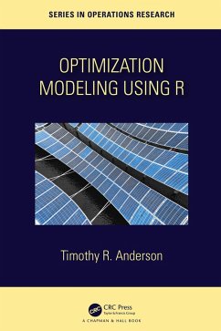
Optimization Modelling Using R (eBook, PDF)
59,95 €
59,95 €
inkl. MwSt.
Sofort per Download lieferbar
30 °P sammeln
59,95 €
Als Download kaufen
59,95 €
inkl. MwSt.
Sofort per Download lieferbar
30 °P sammeln
Jetzt verschenken
Alle Infos zum eBook verschenken
59,95 €
inkl. MwSt.
Sofort per Download lieferbar
Alle Infos zum eBook verschenken
30 °P sammeln
Timothy R. Anderson
Optimization Modelling Using R (eBook, PDF)
- Format: PDF
- Merkliste
- Auf die Merkliste
- Bewerten Bewerten
- Teilen
- Produkt teilen
- Produkterinnerung
- Produkterinnerung
Bitte loggen Sie sich zunächst in Ihr Kundenkonto ein oder registrieren Sie sich bei
bücher.de, um das eBook-Abo tolino select nutzen zu können.
Hier können Sie sich einloggen
Sie sind bereits eingeloggt. Klicken Sie auf 2. tolino select Abo, um fortzufahren.
Bitte loggen Sie sich zunächst in Ihr Kundenkonto ein oder registrieren Sie sich bei bücher.de, um das eBook-Abo tolino select nutzen zu können.
This book covers using R for doing optimization, a key area of operations research, which has been applied to virtually every industry. The focus is on linear and mixed integer optimization. It uses an algebraic modeling approach for creating formulations that pairs naturally with an algebraic implementation in R.
- Geräte: PC
- ohne Kopierschutz
- eBook Hilfe
- Größe: 9.08MB
This book covers using R for doing optimization, a key area of operations research, which has been applied to virtually every industry. The focus is on linear and mixed integer optimization. It uses an algebraic modeling approach for creating formulations that pairs naturally with an algebraic implementation in R.
Dieser Download kann aus rechtlichen Gründen nur mit Rechnungsadresse in A, B, BG, CY, CZ, D, DK, EW, E, FIN, F, GR, HR, H, IRL, I, LT, L, LR, M, NL, PL, P, R, S, SLO, SK ausgeliefert werden.
Produktdetails
- Produktdetails
- Verlag: Taylor & Francis
- Seitenzahl: 298
- Erscheinungstermin: 5. Juli 2022
- Englisch
- ISBN-13: 9781000606843
- Artikelnr.: 63958252
- Verlag: Taylor & Francis
- Seitenzahl: 298
- Erscheinungstermin: 5. Juli 2022
- Englisch
- ISBN-13: 9781000606843
- Artikelnr.: 63958252
Dr. Timothy Anderson is the Department Chair of the Engineering and Technology Management at Portland State University. He earned an Electrical Engineering degree from the University of Minnesota, as well as both M.S. and Ph.D. degrees in Industrial and Systems Engineering from the Georgia Institute of Technology. He leads the Extreme Technology Analytics research group. With over 40 refereed publications, current research interests include analytics, benchmarking, technology forecasting, data mining, and new product development. He is a Sequoyah Fellow of the American Indian Science and Engineering Society. Dr. Anderson is also a past President of Omega Rho, the International Honor Society for Operations Research.
Preface
1 Introduction
1.1 What is Operations Research
1.2 Purpose of this Book
1.3 Range of Operations Research Techniques
1.4 Relationship between Operations Research and Analytics
1.5 Importance of Optimization
1.6 Why R?
1.7 Conventions Used in this Book
2 Introduction to Linear Programming
2.1 What is Linear Programming
2.2 Two Variable Base Case
2.3 Graphically Solving a Linear Program
2.4 Implementing and Solving with ompr
2.4.1 Preparing to Implement the Linear Program
2.4.2 Implementing the Base Case with Piping
2.5 Adding a Third Product (Variable)
2.5.1 Three Variable Base Case Formulation
2.5.2 Three Variable Base Case Implementation
2.5.3 Three Variable Case Results and Interpretation
2.6 Linear Programming Special Cases
2.6.1 Case 1: No Feasible Solution
2.6.2 Case 2: Multiple Optima
2.6.3 Case 3: Redundant Constraint
2.6.4 Case 4: Unbounded Solution
2.7 Abstracting the Production Planning Model
2.8 Methods of Solving Linear Programs
2.9 Exercises
3 More Linear Programming Models
3.1 Types of LP Models
3.2 The Algebraic Model
3.2.1 Tips and Conventions for Algebraic Models
3.2.2 Building the Generalized Model in R
3.2.3 Examining the Results
3.2.4 Changing the Model
3.3 Common Linear Programming Applications
3.3.1 Blending Problems
3.4 Allocation Models
3.4.1 Covering Models
3.4.2 Transportation Models
3.4.3 Transshipment Models
3.4.4 Production and Inventory Planning
3.4.5 Standard Form
3.5 Vector and Matrix Forms of LPs
3.6 Exercises
4 Sensitivity Analysis
4.1 Base Case
4.2 Shadow Prices
4.2.1 Extraction and Interpretation .
4.2.2 Example of Adding an Hour to Assembly
4.2.3 Shadow Prices of Underutilized Resources
4.3 Reduced Costs of Variables
4.3.1 Reduced Cost of Ants
4.3.2 Reduced Price of Bats
4.4 Using Sensitivity Analysis to Evaluate a New Product
4.5 Exercises
5 Data Envelopment Analysis
5.1 Introduction
5.2 Creating the Data
5.3 Graphical Analysis
5.4 The Linear Programs for DEA
5.4.1 An Explicit Linear Program for DEA
5.4.2 A Generalized Linear Program for DEA
5.5 Creating the LP - The Algebraic Approach
5.6 Returns to Scale
5.7 Multiple Inputs and Multiple Outputs
5.8 Extracting Multiplier Weights from Sensitivity Analysis
5.9 Slack Maximization
5.10 DEA Packages
5.11 DEA Model Building
5.11.1 Selection of Inputs and Outputs
5.11.2 Model Choices
5.11.3 Application Area Expertise
5.12 Further Reading
5.13 Exercises
6 Mixed Integer Optimization
6.1 Example of Minor Integrality Impact
6.2 Example of Major Integality Impact
6.3 The Branch and Bound Algorithm
6.3.1 The LP Relaxation
6.3.2 Subproblem I
6.3.3 Subproblem III
6.3.4 Subproblem IV
6.3.5 Subproblem V
6.3.6 Subproblem VI
6.3.7 Subproblem VII
6.3.8 Subproblem VIII
6.3.9 Subproblem II
6.4 Computational Complexity
6.4.1 Full Enumeration
6.5 Binary Variables and Logical Relations
6.6 Fixed Charge Models
6.6.1 Fixed Charge Example-Introduction
6.6.2 Linking Constraints with "Big M"
6.6.3 Fixed Charge Implementation
6.7 Model Results and Interpretation
7 More Integer Programming Models
7.1 Overview
7.2 Revisiting the Warehouse Location Problem
7.2.1 Implementing the Warehouse Model
7.2.2 Solving the Warehouse Location Problem
7.2.3 Warehouse Discussion
7.3 Solving MIPs with Different Solvers
7.3.1 Performance of glpk
7.3.2 Performance of symphony
7.3.3 Performance of lpsolve
7.3.4 Performance of gurobi
7.3.5 Comparing Results across Solvers
7.3.6 Popularity of LP Solvers
7.4 Solving Sudoku Puzzles using Optimization
7.4.1 Introduction to Sudoku and Optimization
7.4.2 Formulating the Sudoku Problem
7.4.3 Implementing Sudoku in ompr
7.4.4 Sudoku Discussion
7.5 Exercises
7.6 Production Planning over Time
7.6.1 Implementing the Model
7.7 Additional Exercises
8 Goal Programming
8.1 Introduction
8.2 Preemptive Goal Programming
8.3 Policies for Houselessness
8.4 Mass Mailings
8.4.1 Formulating the State Mailing Model
8.4.2 Implementing the State Mailing Model
8.4.3 Frontloading the Work
8.5 Exercises
Appendix
A A Very Brief Introduction to R
A.1 Purpose
A.2 Getting Started with R
A.3 Exercises
B Introduction to Math Notation
B.1 Purpose
B.2 Basic Summation Notation
B.3 Using LaTeX in RMarkdown
B.4 Inline Notation
B.5 Sums
B.6 Delimiters
B.7 Summary of Mathematical Notations
B.8 Sequences and Summation Notation
B.9 Applications of Summation
B.10 Double Summation
B.11 Applications of Double Summation
B.12 Exercises
C Troubleshooting
C.1 Overview
C.2 Model Building
C.2.1 Define and Formulate before Implementing
C.2.2 Failing to Look for Past Optimization Models
C.2.3 Misrendering of PDF
C.2.4 Blank Lines in LaTeX
C.2.5 Problems with PDF Creation
C.3 Implementation Troubleshooting
C.3.1 Errors in a Piped Model
C.3.2 Undefined Object in ompr
C.3.3 Unexpected Symbol in ompr
C.3.4 Name Conflicts between R and ompr
C.3.5 Blindly Reusing Code
C.4 General Debugging Tips
C.5 Getting Help
D Making Good Tables 263
D.1 Importance of Tables in Modeling
D.2 Kable vs. Kbl
D.3 Table Footnotes with Kable
D.4 Setting Row and Column Names in Kable
D.5 Booktabs vs. Default
D.6 Using LaTeX in Kable Column Names
D.7 Fitting Tables to Page Width
Bibliography
Index