Brian R Hunt, Ronald L Lipsman, John E Osborn, Jonathan M Rosenberg
Differential Equations with MATLAB
Brian R Hunt, Ronald L Lipsman, John E Osborn, Jonathan M Rosenberg
Differential Equations with MATLAB
- Broschiertes Buch
- Merkliste
- Auf die Merkliste
- Bewerten Bewerten
- Teilen
- Produkt teilen
- Produkterinnerung
- Produkterinnerung
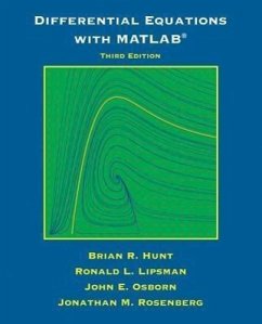
A supplemental text that can enrich and enhance any first course in ordinary differential equations This supplement helps instructors move towards an earlier use of numerical and geometric methods, place a greater emphasis on systems (including nonlinear ones), and increase discussions of both the benefits and possible pitfalls in numerical solution of ODEs. By providing an introduction to the software that is integrated with the relevant mathematics, Differential Equations with MATLAB can perfectly complement and enhance other texts from Wiley. Since the third edition of Differential…mehr
Andere Kunden interessierten sich auch für
![General Linear Methods for Ordinary Differential Equations General Linear Methods for Ordinary Differential Equations]() Zdzislaw JackiewiczGeneral Linear Methods for Ordinary Differential Equations178,99 €
Zdzislaw JackiewiczGeneral Linear Methods for Ordinary Differential Equations178,99 €![Elementary Differential Equations and Boundary Value Problems Elementary Differential Equations and Boundary Value Problems]() William E BoyceElementary Differential Equations and Boundary Value Problems102,99 €
William E BoyceElementary Differential Equations and Boundary Value Problems102,99 €![Advanced Numerical and Semi-Analytical Methods for Differential Equations Advanced Numerical and Semi-Analytical Methods for Differential Equations]() Snehashish ChakravertyAdvanced Numerical and Semi-Analytical Methods for Differential Equations121,99 €
Snehashish ChakravertyAdvanced Numerical and Semi-Analytical Methods for Differential Equations121,99 €![Differential Equations Differential Equations]() James R BrannanDifferential Equations171,99 €
James R BrannanDifferential Equations171,99 €![Principles of Differential Equations Principles of Differential Equations]() Nelson G MarkleyPrinciples of Differential Equations213,99 €
Nelson G MarkleyPrinciples of Differential Equations213,99 €![Elementary Differential Equations Elementary Differential Equations]() William E BoyceElementary Differential Equations172,99 €
William E BoyceElementary Differential Equations172,99 €![Differential Equations Differential Equations]() James R BrannanDifferential Equations296,99 €
James R BrannanDifferential Equations296,99 €-
-
-
A supplemental text that can enrich and enhance any first course in ordinary differential equations This supplement helps instructors move towards an earlier use of numerical and geometric methods, place a greater emphasis on systems (including nonlinear ones), and increase discussions of both the benefits and possible pitfalls in numerical solution of ODEs. By providing an introduction to the software that is integrated with the relevant mathematics, Differential Equations with MATLAB can perfectly complement and enhance other texts from Wiley. Since the third edition of Differential Equations with MATLAB first appeared in 2012, there have been many changes and enhancements to MATLAB and Simulink. These include addition of live scripts, new plotting commands, and major changes to the Symbolic Math Toolbox. This revised version brings the text completely up to date with the 2019a release of MATLAB.
Hinweis: Dieser Artikel kann nur an eine deutsche Lieferadresse ausgeliefert werden.
Hinweis: Dieser Artikel kann nur an eine deutsche Lieferadresse ausgeliefert werden.
Produktdetails
- Produktdetails
- Verlag: Wiley
- 10th Revised edition
- Seitenzahl: 304
- Erscheinungstermin: 24. September 2019
- Englisch
- Abmessung: 233mm x 189mm x 20mm
- Gewicht: 538g
- ISBN-13: 9781118376805
- ISBN-10: 1118376803
- Artikelnr.: 35724448
- Herstellerkennzeichnung
- Libri GmbH
- Europaallee 1
- 36244 Bad Hersfeld
- 06621 890
Brian Hunt and Ronald Lipsman are Professors Emeriti of Mathematics, and Jonathan Rosenberg is Ruth M. Davis Professor of Mathematics, at the University of Maryland. John E. Osborn was Professor Emeritus of Mathematics at the University of Maryland until his death in 2011.
Preface v
1 Introduction 1
1.1 Guiding Philosophy 1
1.2 Student's Guide 3
1.3 Instructor's Guide 5
1.3.1 MATLAB and Simulink 5
1.3.2 ODE Chapters 5
1.3.3 Computer Problem Sets 6
1.4 A Word about Software Versions 7
2 Getting Started with MATLAB 9
2.1 Platforms and Versions 9
2.2 Installation 10
2.3 Starting MATLAB 10
2.4 Typing in the Command Window 11
2.5 Online Help 11
2.6 MATLAB Windows 13
2.7 Ending a Session 14
3 Doing Mathematics with MATLAB 15
3.1 Arithmetic 15
3.2 Symbolic Computation 16
3.2.1 Substituting in Symbolic Expressions 17
3.2.2 Symbolic Expressions and Variable Precision Arithmetic 17
3.3 Vectors 18
3.3.1 Suppressing Output 19
3.4 Recovering from Problems 19
3.4.1 Errors in Input 20
3.4.2 Aborting Calculations 20
3.5 Functions 20
3.5.1 Built-in Functions 20
3.5.2 User-defined Functions 21
3.6 Managing Variables 21
3.7 Solving Equations 23
3.8 Graphics 25
3.8.1 Graphing with fplot 25
3.8.2 Modifying Graphs 26
3.8.3 Graphing with plot 26
3.8.4 Plotting Multiple Curves 28
3.8.5 Parametric Plots 28
3.8.6 Implicit Plots and Contour Plots 29
3.9 Calculus 31
3.10 Some Tips and Reminders 32
4 Using the Desktop and Scripts 33
4.1 The MATLAB Desktop 33
4.1.1 The Workspace 33
4.1.2 The Current Folder and Search Path 34
4.1.3 The Command History 35
4.2 Scripts and Functions 36
4.2.1 Plain Code Scripts 36
4.2.2 Live Scripts 38
4.2.3 Functions 39
4.3 Loops 40
4.4 Presenting Your Results 41
4.4.1 Presenting Graphics 42
4.4.2 Pretty Printing 44
4.4.3 "Publishing" a script 44
4.4.4 Preparing Homework Solutions 45
4.4.5 Exporting a Live Script 46
4.5 Debugging Your Scripts 48
Problem Set A: Practice with MATLAB 51
5 Solutions of Differential Equations 55
5.1 Finding Symbolic Solutions 55
5.2 Existence and Uniqueness 58
5.3 Stability of Differential Equations 60
5.4 Different Types of Symbolic Solutions 63
6 Finer Points of the Symbolic Math Toolbox 69
7 A Qualitative Approach to Differential Equations 75
7.1 Direction Field for a First Order Linear Equation 75
7.2 Direction Field for a Non-Linear Equation 77
7.3 Autonomous Equations 79
7.3.1 Examples of Autonomous Equations 81
Problem Set B: First Order Equations 85
8 Numerical Methods 97
8.1 Numerical Solutions Using MATLAB 98
8.2 Some Numerical Methods 101
8.2.1 The Euler Method 102
8.2.2 The Improved Euler Method 105
8.2.3 The Runge-Kutta Method 106
8.2.4 Inside ode45 107
8.2.5 Round-off Error 108
8.3 Controlling the Error in ode45 108
8.4 Reliability of Numerical Methods 109
9 Features of MATLAB 113
9.1 Data Classes 113
9.1.1 Symbolic and Floating Point Numbers 114
9.1.2 Structures 115
9.1.3 String Manipulation 116
9.2 Functions and Expressions 116
9.3 More about Scripts and Functions 118
9.3.1 Variables and Input/Output in Scripts 118
9.3.2 Variables in Functions 118
9.3.3 Structure of Functions 119
9.4 Matrices 120
9.4.1 Solving Linear Systems 121
9.4.2 Calculating Eigenvalues and Eigenvectors 121
9.5 Graphics 121
9.5.1 Figure Windows and Live Script Graphics 122
9.5.2 Editing Figures 123
9.6 Features of MATLAB's Numerical ODE Solvers 125
9.6.1 Evaluation of Numerical Solutions with deval 125
9.6.2 Plotting Families of Numerical Solutions of ODEs 126
9.6.3 Event Detection 127
9.7 Troubleshooting 129
9.7.1 The Most Common Mistakes 129
9.7.2 Error and Warning Messages 130
10 Using Simulink 133
10.1 Constructing and Running a Simulink Model 133
10.2 Output to the Workspace and How Simulink Works 138
Problem Set C: Numerical Solutions 143
11 Solving and Analyzing Second Order Linear Equations 151
11.1 Second Order Equations with MATLAB 153
11.2 Second Order Equations with Simulink 157
11.3 Comparison Methods 159
11.3.1 The Interlacing of Zeros 160
11.3.2 Proof of the Sturm Comparison Theorem 161
11.4 A Geometric Method 162
11.4.1 The Constant Coefficient Case 163
11.4.2 The Variable Coefficient Case 164
11.4.3 Airy's Equation 165
11.4.4 Bessel's Equation 166
11.4.5 Other Equations 167
Problem Set D: Second Order Equations 169
12 Series Solutions 183
12.1 Series Solutions 184
12.2 Singular Points 186
12.3 Other Linear and Nonlinear Equations 187
13 Laplace Transforms 189
13.1 Differential Equations and Laplace Transforms 191
13.2 Discontinuous Functions 194
13.3 Differential Equations with Discontinuous Forcing 196
Problem Set E: Series Solutions and Laplace Transforms 199
14 Higher Order Equations and Systems of First Order Equations 213
14.1 Higher Order Linear Equations 214
14.2 Systems of First Order Equations 215
14.2.1 Linear First Order Systems 215
14.2.2 Using MATLAB to Find Eigenpairs 218
14.3 Phase Portraits 222
14.3.1 Plotting a Single Trajectory 222
14.3.2 Plotting Several Trajectories 223
14.3.3 Numerical Solutions of First Order Systems 225
14.3.4 A Non-Linear System 227
15 Qualitative Theory for Systems of Differential Equations 229
Problem Set F: Systems of Differential Equations 237
Sample Solutions 255
Index 276

